Uncertainty Quantification - Modelling and Simulation Cookbook

In this chapter we discuss concepts for uncertainty quantification for simulation outcomes.

Objectives:

What is uncertainty and why is it important to quantify it?
How can we quantify and communicate uncertainty?

from typing import Callable

import numpy as np
from math import comb

import scipy
#%matplotlib ipympl
from matplotlib import pyplot as plt
from scipy.integrate import solve_ivp

from modelling_and_simulation_cookbook import PredPreySim

Uncertainty (Definition)¶

Uncertainty refers to epistemic situations involving imperfect or unknown information and arises in partially observable or stochastic or complex or dynamic environments (as well as due to ignorance, indolence, or both Thrun & Norvig (2012)). For modelling and simulation, we distinguish two major sources for uncertainty:

Since we can only model what we can perceive and measure in reality, our image of the real system is generally incomplete. This can have many causes and consequences: Maybe our perception of the causal relationships in reality may be flawed, or our measurements from the real system may be unwittingly inaccurate. Maybe, also the system boundaries that one is inevitably forced to set in order to make sense of the system may also be to blame for the fact that it is not possible to capture the system’s behaviour perfectly. We will furthermore summarise this hidden source of uncertainty as intrinsic or Aleatoric uncertainty Kiureghian & Ditlevsen (2009).

The second source for uncertainty is the modelling process itself, in which the modeller has to make simplifications in order to describe the perceived system in a conceptual and furthermore implemented model. This for example also includes known inaccuracies and limitations of available data used for parametrisation. We will call this sources of uncertainty as model/data or Epistemic uncertainty Kiureghian & Ditlevsen (2009). The main difference to the first source is that, the modeller not only recognises that there is uncertainty regarding a certain system component, but also knows exactly why, since the modeller has consciously decided for the abstraction and simplification steps responsible.

In order to advise a decision-maker effectively, it is important to communicate the implications of uncertainty – regardless of its cause. Only then will they have a complete picture of the situation and be able to plan accordingly.

Case-Study: Weather Forecast¶

Let us take the weather forecast as a thought experiment to illustrate the point.

Aleatoric uncertainty: Even though we have been observing the processes associated with the weather for many centuries, there are still many things we do not yet understand. While the understanding of the atmosphere as a multi-scale system and of the role of scale interactions in determining weather and climate variability has developed strongly Slingo & Palmer (2011) during the last centuries there is still no (and will likely never be) “Grand Unified Theory” which perfectly describes all components of the system.
Epistemic uncertainty:
- Model specification: Simplifications when specifying the differential equations and parameters. Leave out micro-effects or negligibly small factors.
- Numerics: Grid used for numerical computations
- System boundaries: Only a part of the world is depicted at once. We do not regard e.g. anything higher than ....
- Parameters: Parameter values come from inaccurate measurements
- Input: Initial conditions not perfectly known (we cannot measure the weather anywhere at once)

Uncertainty & Stochasticity¶

Clearly, stochasticity is the key to incorporate uncertainty in simulation results. There are, in principle, three concepts for integrating stochasticity (see Figure below): (a) Inherently stochastic models, e.g. discrete event models or agent-based models, integrate stochasticity by default. However, there is not guarantee that this covers all uncertainty involved and one should also consider adding additional stochasticity at other points. (b) Input and (c) parameter uncertainty can be incorporated by stochastically varying input (e.g. initial conditions) and parameter values. Clearly (a), (b) and (c) can be combined as well.

Anyhow, in all three cases we find, that the model’s states and in particular outputs, are no longer deterministic (e.g. a scalar, a vector or a function of time) but are instead a random variable (e.g. scalar-valued, vector-valued or stochastic process).

Quantification of Uncertainty¶

As already mentioned, quantifying the uncertainty associated with the model is crucial to ensuring that the results can be used as effectively as possible as a basis for decision-making.

Case-Study: Manufacturing - Analytic¶

We illustrate this by a very simple case study: Let us assume that a company manufactures a certain product and wishes to sell it. During production, there is a probability $0<p\ll 1$ that a fault will occur, rendering the product unsaleable. It is clear that the firm’s expected revenue $R$ from the production of $N$ products is

\mathbb{E}(R)=N(1-p)c,

(1)

where $c$ is the selling price of a product, assuming that all viable products will be sold. However, this information does not incorporate the corresponding uncertainty and is therefore insufficient for planning.

Since the sum of Bernoulli distributed (i.e. either zero or one) random variables is known to follow a Binomial distribution, we may compute the individual probabilities

k\in \{0,\dots,N\}: P(R=ck)=c\left(\begin{array}{c}N\\k\end{array}\right)(1-p)^kp^{N-k}

(2)

and use this information to specify regions of confidence. For example, defining

k_{q}:=\max_{k\in \{0,\dots,N\}}:\sum_{k=0}^{k_{q}}P(R=ck)<1-q

(3)

we find that wth $100q\%$ certainty, the manufacturing of $N$ products will yield a revenue of at least $ck_{q}$ .

With this additional information, the decision-maker is now better placed to plan, e.g. future expenditures. How they choose to do this is now down to their willingness to take risks.

The situation is implemented below.

p = 0.02 # probability of failure
N = 20 # products (note that "comb" is only possible for rather small values of N)
c = 9 # price of the product

r_avg = N*(1-p)*c # expected value
print(f'expected revenue {r_avg}')

# compute the probability for every possible outcome
r_prob = list()
for k in range(N+1):
    r_prob.append(comb(N,k)*(1-p)**k*p**(N-k))

def get_min_revenue(r_prob:list[float],q:float) -> float:
    """
    Returns the minimum revenue with given confidence q
    :param r_prob: vector of probabilities
    :param q: confidence
    :return:
    """
    sm = 0
    for k,p in enumerate(r_prob):
        sm+=p
        if sm>(1-q):
            return k*c
    return len(r_prob)*c

q = 0.90 # confidence level
r_q = get_min_revenue(r_prob,q)
print(f'minimum revenue ({100*q:.0f}% certainty): {r_q}')
q = 0.99
r_q = get_min_revenue(r_prob,q)
print(f'minimum revenue ({100*q:.0f}% certainty): {r_q}')

expected revenue 176.4
minimum revenue (90% certainty): 171
minimum revenue (99% certainty): 162

Case-Study: Manufacturing - Monte Carlo¶

The prior analysis was based on the important property that the distribution of the revenue, i.e. the Binomial distribution, was analytically known and understood. However, in the general case this is not possible and one needs to rely on numerical approximations.

Clearly, the Monte Carlo Method / Simulation, as introduced in chapter Monte Carlo Simulation is the key to this. While it is originally designed to estimate the unknown mean value of the distribution (by the sample mean), it does, per se, not limit itself to any specific statistic and can be used to estimate arbitrary moments, confidence intervals or entire distributions. Below, the revenue problem is solved using a Monte Carlo approach.

p = 0.02 # probability of failure
N = 20 # products (no limitations here)
c = 9 # price of the product

mc_iterations = 10000 #monte-carlo runs

np.random.seed(12345)
samples = list()
for i in range(mc_iterations):
    # run the experiment
    successes = [np.random.random()>p for x in range(N)]
    samples.append(sum(successes)*c)

r_avg = sum(samples)/len(samples) # sample mean
print(f'expected revenue {r_avg}')
q = 0.90 # confidence level
r_q = np.quantile(samples,1-q)
print(f'minimum revenue ({100*q:.0f}% certainty): {r_q}')
q = 0.99
r_q = np.quantile(samples,1-q)
print(f'minimum revenue ({100*q:.0f}% certainty): {r_q}')

expected revenue 176.4081

minimum revenue (90% certainty): 171.0
minimum revenue (99% certainty): 162.0

Case-Study: Predator-Prey model¶

To study uncertainty quantification we will use the predator-prey model from Chapter Simulation Circle as a case study whilst disregarding the modelling of the intervention. The model is defined as a system of two coupled differential equations

\frac{dx}{dt}(t)=x(t)(\alpha_1-\beta_1)-x(t)y(t)\gamma,

(4)

\frac{dy}{dt}(t)=y(t)(\alpha_2-\beta_2)+x(t)y(t)\gamma\delta.

(5)

and has six parameters $\alpha_1,\beta_1,\alpha_2,\beta_2,\gamma,\delta$ . The two cuves $x$ and $y$ descibe the population size of a prea and predator species and $\alpha_{1/2}$ and $\beta_{1/2}$ are the corresponding reproduction and death rates. In the model they actually only enter as their respective differences whereas the model leads to traditional predator-prey behaviour when $\alpha_1>\beta_1$ and $\alpha_2<\beta_2$ . The parameters $\gamma$ and $\delta$ influence the interaction between the species in terms of one hunting and eating the other.

For the case study we fix

\alpha_1=0.2,\beta_1=0.1,\alpha_2=0.1,\beta_2=0.3,\text{ and }\delta=1.

(6)

To incorporate uncertainty we further specify, that neither initial values nor interaction terms between the two species are perfectly known. We define

\gamma\sim \mathcal{N}(0.3,0.02),x(0)=x_0\sim\mathcal{N}(0.5,0.02),\text{ and } y(0)=y_0\sim\mathcal{N}(0.1,0.01)

(7)

and capture the uncertainty using Monte-Carlo simulation with $M=1000$ samples.

alpha_1 = 0.2
beta_1 = 0.1
alpha_2 = 0.1
beta_2 = 0.3
delta = 1.0
gamma_mean = 0.3
gamma_std = 0.02
prey0_mean = 0.5
prey0_std = 0.02
predator0_mean = 0.1
predator0_std = 0.01

def mc_run() -> tuple[np.ndarray,np.ndarray,np.ndarray]:
    """
    Performs a single monte-carlo run.
    """
    prey0 = np.random.normal()*prey0_std+prey0_mean
    predator0 = np.random.normal()*predator0_std+predator0_mean
    gamma = np.random.normal()*gamma_std+gamma_mean
    sim = PredPreySim(alpha_1,beta_1,alpha_2,beta_2,gamma,delta)
    return sim.run(100,prey0,predator0)

mc_iterations = 1000
np.random.seed(12345)
results = list()
for i in range(mc_iterations):
    t,prey,pred = mc_run()
    results.append((t,prey,pred))

def plot_individual_runs(prey_plot:bool=True,predator_plot:bool=True):
    """
    Plots the individual resuls of the MC simulation
    :param prey_plot: if prey lines should be plotted
    :param predator_plot: if predator lines should be plotted
    """
    for t,prey,pred in results:
        if prey_plot:
            plt.plot(t,prey,color=[0,0.1,0],linewidth=0.05)
        if predator_plot:
            plt.plot(t,pred,color=[0,0,0.1],linewidth=0.05)

plt.figure(figsize=(10,5))
plot_individual_runs()
plt.show()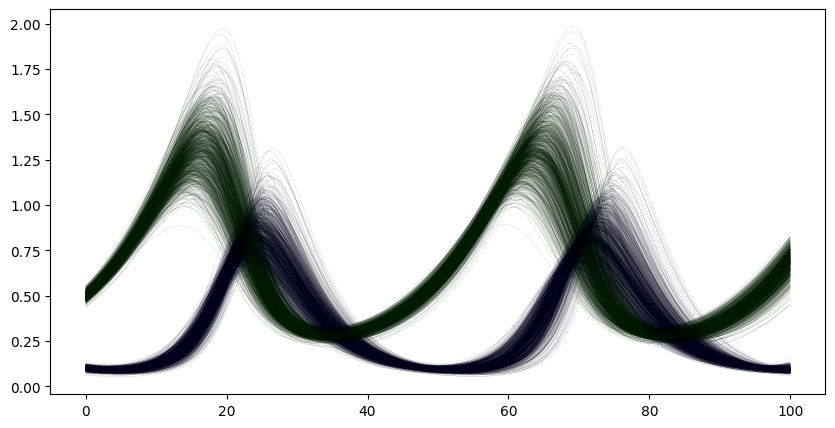

The results of the predator-prey simulation are two timeseries, one for the prey and one for the predators, which are given for the common time-base $[0,1,\dots,T]$ . That means, the $M$ results $\vec{x}_1,\dots,\vec{x}_M$ of the simulation are observations of a random vector $\vec{X}\in \left(\mathbb{R}^+\right)^{2(T+1)}$ , in which the first $T+1$ entries represent the quantity of prey animals for times $[0,1,\dots,T]$ and the second the predator animals.

The most straight forward statistic that can be calculated from the results is the point-wise sample mean $\overline{X}_M$ which approximates the unknown real mean $\vec{\mu}=\mathbb{E}(\vec{X})$ , i.e.

\vec{\mu}\approx \overline{X}_M = \frac{1}{M}\sum_{i=1}^{M}\vec{x}_i.

(8)

By this point at the latest, one must be clear about the outcomes of interest. Suppose $\vec{Y}=f(\vec{X})$ is a derived outcome, then

\mathbb{E}(f(\vec{X}))\text{ and }f\left(\mathbb{E}(\vec{X})\right)

(9)

are generally not equivalent. One example for the given case study is the maximum peak height:

f(\vec{X})=\left(\begin{array}{c}max\left(\vec{X}_{1}^{T+1}\right)\\max\left(\vec{X}_{T+2}^{2(T+1)}\right)\end{array}\right)

(10)

for which $\mathbb{E}(f(\vec{X}))\neq f\left(\mathbb{E}(\vec{X})\right)$ .

prey_array = np.array([x[1] for x in results]) # make statistics easier
predator_array = np.array([x[2] for x in results]) # make statistics easier
time_array = results[0][0]
sample_mean = (results[0][0], np.average(prey_array,axis=0),np.average(predator_array,axis=0))

def plot_sample_mean() -> None:
    """
    Plots the pointwise sample mean
    """
    plt.plot(time_array,sample_mean[1],color=[1.0,0.2,0],label='prey (mean)')
    plt.plot(time_array,sample_mean[2],color=[1.0,0,0.2],label='predator (mean)')

plt.figure(figsize=(10,5))
plot_individual_runs()
plot_sample_mean()
plt.show()

f_of_mean = (max(sample_mean[1]),max(sample_mean[2])) # compute peak heights of mean

fs = [np.max(prey_array,axis=1),np.max(predator_array,axis=1)] # compute individual peaks
mean_of_fs = [np.average(fs[0]),np.average(fs[1])] # compute mean of peaks
print(f'peaks of mean: {f_of_mean}')
print(f'mean of peaks: {mean_of_fs}')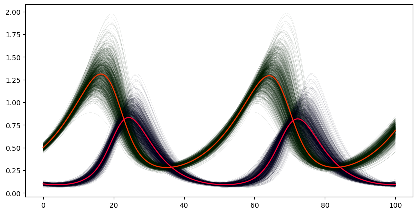

peaks of mean: (np.float64(1.3122723575543607), np.float64(0.8329920238429047))
mean of peaks: [np.float64(1.328956837488559), np.float64(0.8457135478131288)]

While the values are not far apart, they are clearly not equivalent. One lession here is that one should be careful when discarding the individually computed results from a Monte Carlo simulation. Retrospective calculation of statistics for derived outcomes may become impossible.

Finally, it is important to observe, for the same reason as before, that the mean of the simulation results is not necessarily equivalent to the (deterministic) simulation executed for the mean of the inputs.

sim = PredPreySim(alpha_1,beta_1,alpha_2,beta_2,gamma_mean,delta) # model with parameter gamma averag
t_input_mean,prey_input_mean,predator_input_mean = sim.run(100,prey0_mean,predator0_mean) # run with initial value average
plt.figure(figsize=(10,5))
plot_sample_mean()
plt.plot(t_input_mean,prey_input_mean,color=[0.2,0,1],label='prey (input mean)')
plt.plot(t_input_mean,predator_input_mean,color=[0,0.2,1],label='predator (input mean)')
plt.legend()
plt.show()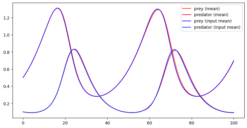

Quantification of Uncertainty¶

Now that we can calculate the expected value, it is time to quantify the uncertainties associated with the distribution. Given a list of results $\vec{x}_1,\dots,\vec{x}_M$ there are essentially two different approaches: parametric and non-parametric.

Uncertainty using Parametric Statistics¶

This parametric approach is based on the assumption that the results pointwise follow a known distribution $\mathcal{D}$ with parameters $p_1,\dots,p_k$ to be determined. We estimate the parameters from the individual Monte Carlo samples and use analytic knowledge from the distribution to quantify uncertianty measures such as confidence intervals.

The most common choice for such a distribution is the normal distribution $\mathcal{N}(\mu,\sigma)$ with the two parameters mean $\mu$ and standard deviation $\sigma$ . This choice is particularly popular because it is often a reliable fit, and estimation of the parameters is quite simple: we already calculated the pointwise sample mean $\vec{X}_M$ and computation of the sample variance (and standarddeviation) is hardly more complicated:

\vec{\sigma}^2\approx\vec{s}_M^2=\frac{1}{M-1}\sum_{i=1}^{M}(\vec{x}_i-\vec{X}_M)^2,

(11)

whereas all computations must be understood pointwise. The factor $\frac{1}{M-1}$ instead of $\frac{1}{M}$ is used to make the estimator free of bias.

For a $\mathcal{N}(\mu,\sigma)$ normally distributed $X$ we know

P\left(X<\mu-\sigma\Phi^{-1}(p)\right)=p

(12)

wheras $\Phi^{-1}$ is the inverse of the cumulative distribution function. As a result

\left[\mu-\Phi^{-1}(p)\sigma,\mu+\Phi^{-1}(p)\sigma\right]\approx \left[\overline{X}_M-\Phi^{-1}(p)\sqrt{\vec{s}^2_M},\overline{X}_M+\Phi^{-1}(p)\sqrt{\vec{s}^2_M}\right]

(13)

is a $100(1-2(1-p))\%$ confidence interval.

sample_variance = (time_array, np.var(prey_array,axis=0),np.var(predator_array,axis=0))
sample_std = np.sqrt(sample_variance)
p = 0.95
z = scipy.stats.norm.ppf(p)
plt.figure(figsize=(10,5))
plt.fill_between(time_array,sample_mean[1]-sample_std[1]*z,sample_mean[1]+sample_std[1]*z,color=[1.0,0.2,0.0],alpha=0.3,label=f'prey ({100*(1-2*(1-p)):.0f}% CI)')
plt.fill_between(time_array,sample_mean[2]-sample_std[2]*z,sample_mean[2]+sample_std[2]*z,color=[1.0,0.0,0.2],alpha=0.3,label=f'predator ({100*(1-2*(1-p)):.0f}% CI)')
plot_sample_mean()
plt.legend()
plt.show()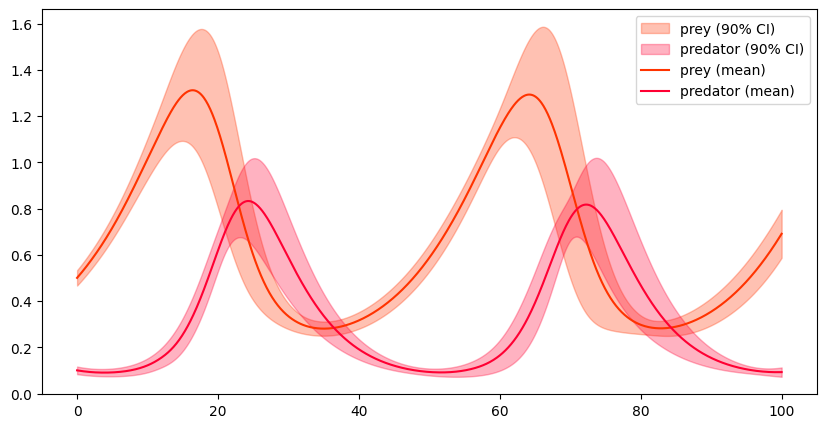

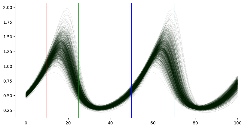
The confidence interval relies on the assumption that the Monte Carlo runs do indeed follow the given distribution. It is advisable to verify this on a random basis, for example by using a Gaussian kernel density estimatation (KDE) to estimate the empirical density.

ts = [10,25,50,70]
colors = ['r','g','b','c']

plt.figure(figsize=(10,5))
plot_individual_runs(predator_plot=False)

yl = plt.ylim() # get original y-lims
for t,c in zip(ts,colors):
    plt.plot([t,t],yl,color=c) # just plot some vertical lines where we want to compute the distribution
plt.ylim(yl) # reset to original y-lims

plt.figure(figsize=(10,10))
for i,t in enumerate(ts):
    c = colors[i]
    plt.subplot(2,2,i+1)
    index = np.where(time_array==t)[0][0] # get the correct index (only works since all values are integers anyway)
    kde = scipy.stats.gaussian_kde(prey_array[:,index]) # get the empirical distribution
    mn = min(prey_array[:,index]) # get limits for the plot
    mx = max(prey_array[:,index]) # get limits for the plot
    x_array = np.linspace(mn,mx,200)
    kde_array = kde.evaluate(x_array) # evaluate the kde
    plt.plot(x_array,kde_array,color=c,linestyle='dashed',label='prey (empirical KDE)')
    gauss_array = scipy.stats.norm.pdf(x_array,loc=sample_mean[1][index],scale=sample_std[1][index]) # compute the density of the normal distribution
    plt.plot(x_array,gauss_array,color=c,label='prey (normal dist.)')
    plt.legend()
    plt.title(f'time {t}')

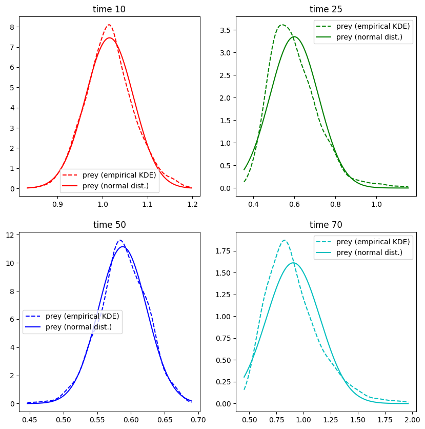
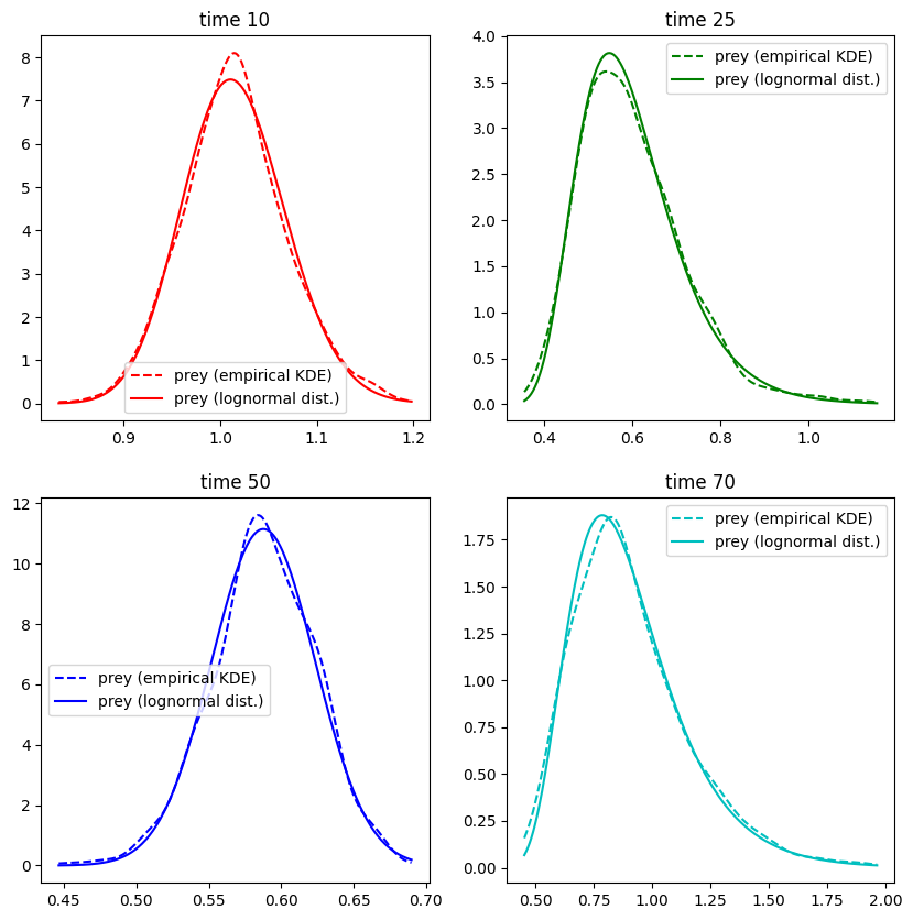
It is well visible, that the distribution is quite skewed in particular when the curves are peaking. A log-normal distribution might be a better fit. Hereby $X\sim Lognormal(\mu,\sigma^2)$ is defined by

X=e^{\mu+\sigma Z}

(14)

where $Z$ follows a standard normal distribution. Since

\mathbb{E}(X)=e^{(\mu+\sigma^2/2)},\text{ and }\mathbb{V}(X)=(e^{\sigma^2}-1)e^{2\mu+\sigma^2}

(15)

we may estimate the two parameters $\mu$ and $\sigma$ from the empirical mean and variance via

\mu=ln\left(\frac{\overline{X}_M^2}{\sqrt{\overline{X}_M^2+s_M^2}}\right),\text{ and } \sigma^2=ln\left(1+\frac{s_M^2}{\overline{X}_M^2}\right).

(16)

Alternatively, it is also possible to automatically fit the distribution using a maximum likelihood method, as done below using lognorm.fit.

plt.figure(figsize=(10,10))
for i,t in enumerate(ts):
    c = colors[i]
    plt.subplot(2,2,i+1)
    index = np.where(time_array==t)[0][0] # get the correct index (only works since all values are integers anyway)
    kde = scipy.stats.gaussian_kde(prey_array[:,index]) # get the empirical distribution
    mn = min(prey_array[:,index]) # get limits for the plot
    mx = max(prey_array[:,index]) # get limits for the plot
    x_array = np.linspace(mn,mx,200)
    kde_array = kde.evaluate(x_array) # evaluate the kde
    plt.plot(x_array,kde_array,color=c,linestyle='dashed',label='prey (empirical KDE)')
    shape,loc,scale = scipy.stats.lognorm.fit(prey_array[:,index]) #maximum likelihood fit
    lognormal_array = scipy.stats.lognorm.pdf(x_array,shape,loc,scale) # compute the density of the lognormal distribution
    plt.plot(x_array,lognormal_array,color=c,label='prey (lognormal dist.)')
    plt.legend()
    plt.title(f'time {t}')
plt.show()
# compute confidence bands
plt.figure(figsize=(10,5))
p = 0.9
for i,array in enumerate([prey_array,predator_array]):
    fitted_parameters = [scipy.stats.lognorm.fit(array[:,i]) for i in range(len(time_array))] # fit for all points in time
    lower_bound = [scipy.stats.lognorm.ppf((1-p)/2,shape,loc=loc,scale=scale) for shape,loc,scale in fitted_parameters]
    upper_bound = [scipy.stats.lognorm.ppf(1-(1-p)/2,shape,loc=loc,scale=scale) for shape,loc,scale in fitted_parameters]
    c = [1.0,0.2,0.0] if i==0 else [1.0,0.0,0.2]
    lbl = 'prey' if i==0 else 'predator'
    plt.fill_between(time_array,lower_bound,upper_bound,color=c,alpha=0.3,label=f'{lbl} ({100*p:.0f}% CI)')
    plt.fill_between(time_array,lower_bound,upper_bound,color=c,alpha=0.3,label=f'{lbl} ({100*p:.0f}% CI)')
plot_sample_mean()
plt.legend()
plt.show()

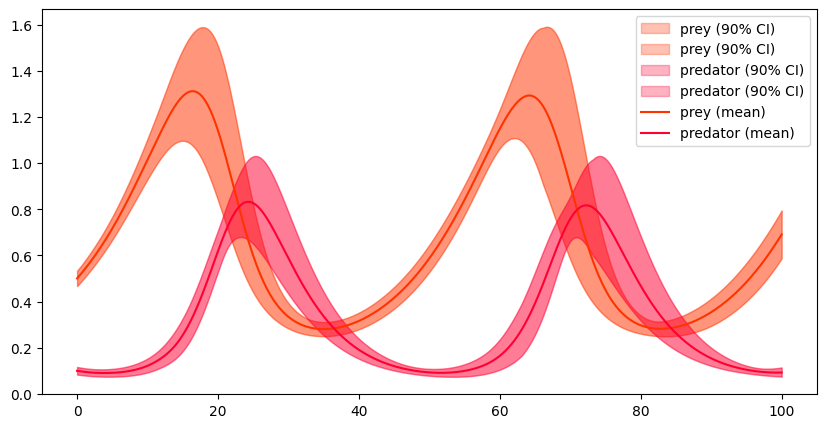
With the log-normal distributions the confidence bands are no longer symmetric which fits the real behaviour much better. Nevertheless, we must ask why we needed a proper distribution assumption in the first place. This motivates the idea for non-parametric approaches.

Uncertainty using Non-Parametric Statistics¶

The most generic approach to use non-parametric statistics for computation of confidence bands are the empirical quantiles. Loosely speaking we can say that a value $q$ is an empirical $p$ -quantile for a sample $x_1,\dots,x_M$ if

|i:x_i\leq q|\approx p\cdot M.

(17)

For example, if $p=0.5$ and $M=101$ is uneven then the $51^{st}$ element of the ordered sample would be the unique proper choice for $q$ . However, if $M=100$ any value greater the $50^{th}$ and smaller than the $51^{st}$ element would be eligible. Unfortunately, there is no unique solution what to do in these cases, most software packages including the numpy.quantile function compute an interpolation between the two values.

The $p=0.5$ quantile is generally called the median and states that the random variable is smaller or larger with equal likelihood. While it is usally in the proximity of mean, it is only equivalent in case of symmetric distributions. The $p=0.25$ and $p=0.75$ quantiles are called quartiles and the span between the two is called interquartile range. It is a well established measure for uncertainty and, together with the median, the foundation of box-plots.

plt.figure(figsize=(10,5))
p = 0.9
for i,array in enumerate([prey_array,predator_array]):
    bounds = np.quantile(array,[(1-p)/2,0.5,1-(1-p)/2],axis=0) # lower-bound, median, upper-bound
    c = [1.0,0.2,0.0] if i==0 else [1.0,0.0,0.2]
    lbl = 'prey' if i==0 else 'predator'
    plt.fill_between(time_array,bounds[0,:],bounds[2,:],color=c,alpha=0.3,label=f'{lbl} ({100*p:.0f}% CI)')
    plt.plot(time_array,bounds[1,:],color=c,linestyle='dashed',label=f'{lbl} (median)')
plot_sample_mean()
plt.legend()
plt.show()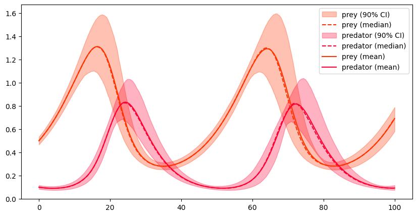

Parametric or Non-Parametric¶

In principle, it is quite easy to choose between the two approaches. On the one hand, estimating confidence bands using quantiles is significantly more robust and always yields values within meaningful ranges. Moreover they do not require any assumptions on the underlying distribution. Unfortunately, they also require a comparably large sample size. If the number of sample is too small, corresponding curves may become very edgy and volatile. E.g. if $M=100$ computing a $p=0.01$ quantile relies on the value of the single smallest sample, which is clearly unstable.

On the other hand, parametric statistics can produce meaningful results even for smaller sample sizes (e.g. Conover (1999)). While $M=100$ can be too small to estimate the quantile, it might be sufficient to estimate a standard deviation or to fit a distribution in general. Knowledge of the distribution properties and parameters can then provide additional informative value, such as tail behaviour or possibilities for extrapolation. However, a parametric estimate is only as good as the fit of the distribution. If the assumption regarding the distribution of the results is poor, the quantified uncertainty will also be incorrect.

Case-Study: Nonlinear-ODE - Proper Statistics?¶

We conclude this topic on uncertainty quantificatuon with a fictional case study. We assume that the dynamics of a system is described by the following non-linear initial-value problem:

\dot{x}=-x(x-2)(x-\alpha), x(0)=x_0=1.0.

(18)

To incproporate uncertainty, we use $\alpha \sim \mathcal{N}(1,0.02)$ and perform $M=1000$ samples.

M = 500 # MC samples
rhs_alpha = lambda t,x,alpha:-x*(x-2)*(x-alpha) # right-hand side function
alpha_mean = 1.0 # mean for input uncertainty
alpha_std = 0.02 # std for input uncertainty
x0 = [1.0] # initial value

# perform MC samples
np.random.seed(12345)
tend = 20
t_eval = np.linspace(0,tend,100)
results = list()
plt.figure(figsize=(10,10))
ax = plt.subplot(2,2,1)
for i in range(M):
    alpha = np.random.normal(loc=alpha_mean,scale=alpha_std)
    rhs = lambda t,x: rhs_alpha(t,x,alpha)
    res = scipy.integrate.solve_ivp(rhs,[0,tend],y0=x0,t_eval=t_eval)
    results.append(res.y[0])
    plt.plot(t_eval,res.y[0],color='k',linewidth=0.1) # plot individual result
plt.title('individual runs')
results = np.array(results)

# compute uncertainty interval with parametric approach (normal distribution)
p = 0.9
plt.subplot(2,2,2,sharey = ax)
sample_mean = np.average(results,axis=0)
sample_variance = np.var(results,axis=0)
sample_std = np.sqrt(sample_variance)
z = scipy.stats.norm.ppf(1-(1-p)/2)
plt.fill_between(t_eval,sample_mean-z*sample_std,sample_mean+z*sample_std,color='r',alpha=0.2,label=f'{100*p:.0f}% CI (Gaussian)')
plt.plot(t_eval,sample_mean,color='r',label='sample mean')
plt.legend()
plt.title('Parametric uncertainty estimate')

# compute uncertainty interval with non-parametric approach
plt.subplot(2,2,3,sharey = ax)
bounds = np.quantile(results,[(1-p)/2,0.5,1-(1-p)/2],axis=0)
plt.fill_between(t_eval,bounds[0],bounds[2],color='r',alpha=0.2,label=f'{100*p:.0f}% CI (empiric quantiles)')
plt.plot(t_eval,bounds[1],color='r',label='median')
plt.legend()
plt.title('Non-parametric uncertainty estimate')

# split the results into upper and lower bundle
# compute uncertainty interval with non-parametric approach
plt.subplot(2,2,4,sharey = ax)
part1 = results[results[:,-1]>1,:]
part2 = results[results[:,-1]<=1,:]
print(f'Probability to be in part 1: {len(part1)/M:.04f}')
for part in [part1,part2]:
    bounds = np.quantile(part,[(1-p)/2,0.5,1-(1-p)/2],axis=0)
    plt.fill_between(t_eval,bounds[0],bounds[2],color='r' if part is part2 else 'b',alpha=0.2,label=f'{100*p:.0f}% CI (quantiles, part2)' if part is part2 else f'{100*p:.0f}% CI (quantiles, part1)')
    plt.plot(t_eval,bounds[1],color='r' if part is part2 else 'b',label='median (part2)' if part is part2 else 'median (part1)')
plt.legend()
plt.title('Non-parametric uncertainty estimate (splitted)')
plt.show()

Probability to be in part 1: 0.5080

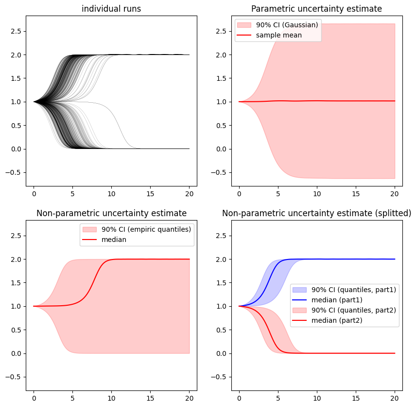
This fictional case study teaches us the important lesson that it is always important to choose the statistics carefully. The differential equation has a so-called bifurcation point at $\alpha$ . For $x(t)<\alpha$ , the solution falls towards $x\equiv 0$ , for $x(t)>\alpha$ , the solution approaches $x\equiv 2$ . Since $\alpha$ is distributed around the initial value $x_0=1$ this means that the solution curves are divided almost perfectly into two parts: one part in which the curves tend towards 0 and another in which they converge towards 2.

Plots 2 and 3 show that any statistical analysis carried out on the entire set of solution curves is virtually meaningless. The mean is almost exactly $x\equiv 1$ and is therefore not representative for any curve; the median is some arbitrary curve which goes up or down basically by coinflip. The standard deviation is enormous and the corresponding Gaussian interval is many times larger than the entire set of curves. Finally, also the empirical interval is also virtually meaningless. Only when the set of curves is divided properly, it is possible to perform proper analysis of the results.

It is therefore recommended that a statistical analysis should always be accompanied by a plot of the individual Monte Carlo runs in order to avoid such errors.

References¶

Thrun, S., & Norvig, P. (2012). Introduction to artificial intelligence. Retrieved March, 19, 2012.
Kiureghian, A. D., & Ditlevsen, O. (2009). Aleatory or epistemic? Does it matter? Structural Safety, 31(2), 105–112. 10.1016/j.strusafe.2008.06.020
Slingo, J., & Palmer, T. (2011). Uncertainty in weather and climate prediction. Philosophical Transactions of the Royal Society A: Mathematical, Physical and Engineering Sciences, 369(1956), 4751–4767. 10.1098/rsta.2011.0161
Conover, W. J. (1999). Practical nonparametric statistics. john wiley & sons.