Monte Carlo Simulation

In this chapter we illustrate the idea of Monte Carlo simulation and how to correctly apply it

Objectives:

How and why does Monte Carlo simulation work?
How do I properly setup a Monte Carlo experiment?
How many samples should I make?

from typing import Callable

import numpy as np
import scipy
#%matplotlib ipympl
from matplotlib import pyplot as plt
from scipy.interpolate import interp1d

from modelling_and_simulation_cookbook import DESSimulator, MultipleServerQueue, RunEvent

Monte Carlo Method¶

The so-called Monte Carlo method is founded on the simple idea that we may gain insights into a given unknown distribution, as soon as one has sufficiently many independently drawn samples $X_i,i\in\{1,\dots,M\}$ from it. Above all, this refers to the estimation of its unknown average value $\mu$ by the sample mean $\overline{X}_M$ , i.e.

\mu:=\mathbb{E}(X)\approx \overline{X}_M:=\frac{1}{M}\sum_{i=1}^{M}X_i,

(1)

which is also known as the Law of Large numbers Dekking et al. (2005).

The term Monte Carlo dates back to the Manhattan project. This project was originally motivated by research into nuclear fission during the Second World War, but the unique coming together of the finest researchers and technology of the time led to countless further innovations (What a pity that a war seems necessary to launch such revolutionary scientific endeavors, N Metropolis). According to Metropolis (1987) invention of the Monte Carlo method was thanks to an idea by Stanislas Ulam, a mathematician with an affinity to stochastic processes and card games, that the concept of stochastic sampling could be linked to the then entirely new possibilities for sampling random numbers offered by the first computers. What was initially tested for calculating the odds of winning in solitaire and other simple games soon found applications in particle physics. In recognition of Ulam’s contribution, corresponding part of the project was subsequently named Project Monte Carlo after Ulam’s grandfather’s favourite casino. Note, that the scientists formally used John von Neumann’s mid-square method, see Pseudo Random Number Generation, to generate the required pseudo random numbers.

Case-Study: Buffon Needle Problem¶

Unlike the computational method, the idea of generating insights into a distribution by sampling is much older. One of the most famous for and commonly believed to be the fist usage of a Monte Carlo method in general dates back to natural scientist George Louise Leclerc de Buffon 1707-1788 Daudin (1801). The famous Buffon Needle Problem is defined as an experimental setup to approximate probabilities:

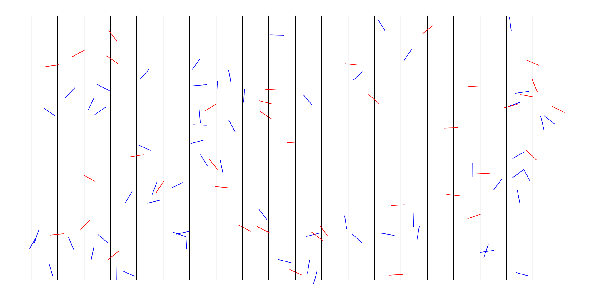
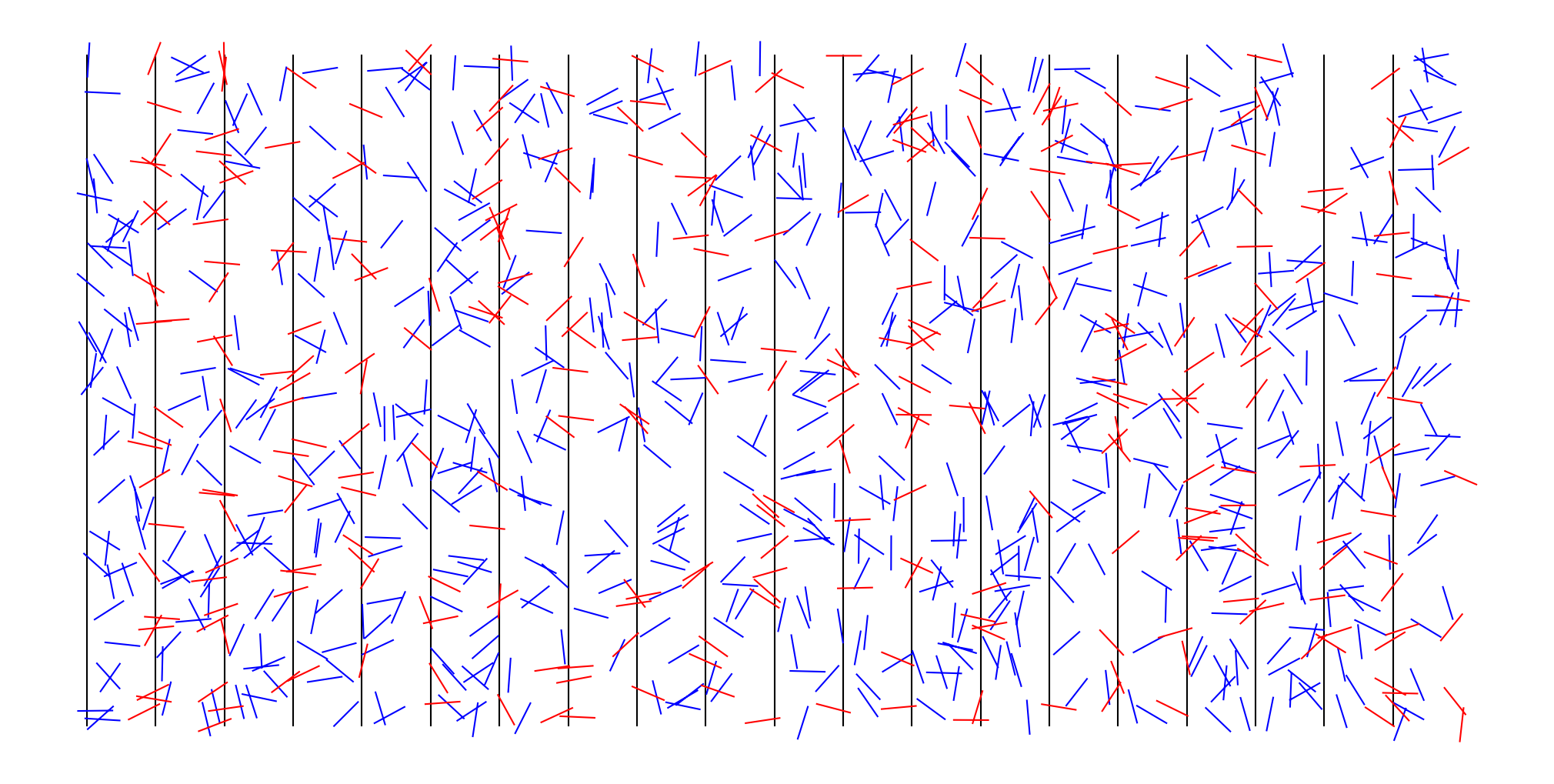
Suppose we have an (infinite) floor vertically tiled by lines into equivalent strips of width $a$ . Now, assume we randomly drop a needle (stick/staff/...) with length $b< a$ and negligible width on it. Let random variable $X$ stand for the event that the dropped stick will intersect with one of the lines ( $X=1$ ) or not ( $X=0$ ). Aim of the experiment is to compute

\mathbb{E}(X)=1\cdot P(X=1)+0\cdot P(X=0)=P(X=1).

(2)

(a) Analytic Due to the comparable simple design of the study, there is a way to compute the probability using (rather) standard calculus. It computes to

P(X=1)=\frac{2b}{a\pi}.

(3)

One way to get to this result is given by the image below. The outcome of $X$ can be seen to depend on two things: (1) the horizontal position of the midpoint of the needle and (2) the needle’s rotation. Note that the vertical position of the needle does not matter due to the tiling. Suppose the rotation $\alpha$ is given, the question if the needle overlaps relates to the cosine of the angle (compare left and right of in the figure). To be precise, there is a zone with width $\frac{b}{2}\cos(\alpha)$ to the left and to the right of any of the lines, in which the needle intersects, and a zone of width $a-b\cos(\alpha)$ in which the needle does not intersect. That means

P(X=1|\alpha) = \frac{b}{a}|\cos(\alpha)|.

(4)

Furthermore, randomly dropping a needle causes a uniformly distributed angle, i.e. $\alpha\sim U(0,2\pi)$ with probability density $\frac{1}{2\pi}$ . As a result, we compute the overall probability by the law of total probability

P(X=1)=\int_{0}^{2\pi}P(X=1|\alpha) dP(\alpha)=\int_{0}^{2\pi}P(X=1|\alpha) \frac{1}{2\pi}d\alpha =\int_{0}^{2\pi}\frac{b}{a}|\cos(\alpha)|\frac{1}{2\pi}d\alpha

(5)

=\frac{b}{2a\pi}\int_{0}^{2\pi}|\cos(\alpha)|\underbrace{=}_{\text{symmetry of cos}}\frac{4b}{2a\pi}\int_{0}^{\pi/2}\cos(\alpha)d\alpha=\frac{4b}{2a\pi}[\sin(\alpha)]_{0}^{\pi/2}=\frac{4b}{2a\pi}=\frac{2b}{a\pi}.

(6)

(b) Monte Carlo The as an alternative, Buffon proposed to drop the needle $M$ times (or carefully dropping multiple needles at a time) counting the total number of overlaps $K_M$ . As a result of the Large Number Theorem, we know that

\lim_{m\rightarrow \infty}\frac{K_M}{M}=\mathbb{E}(X)=P(X=1)=\frac{2b}{a\pi},

(7)

or, from a different perspective,

\frac{K_M}{M}\approx\frac{2b}{a\pi}\Leftrightarrow \frac{2bM}{aK_M}\approx \pi,

(8)

when $M$ is sufficiently large. Long story short, we found a process to approximate $\pi$ .

a = 1 # distance between the lines
b = 0.5 # length of a needle (must be shorter or equal to a)
x_size = 20 # depicted lengh of the floor
y_size = 10 # depicted width of the floor

def drop_needle()->tuple[np.ndarray,np.ndarray]:
    """
    Randomly drops a needle on the floor.
    :return: Start and endpoint of the needle as numpy arrays with two entries
    """
    mid = np.random.random(2)*np.array([x_size,y_size])
    angle = 2*np.pi*np.random.random()
    vec = b/2*np.array([np.cos(angle),np.sin(angle)])
    return mid-vec,mid+vec

def perform_buffon_experiment(needles:int,plot:bool=True) -> int:
    """
    Performs a buffon needle experiment with given number of needles
    :param needles:
    :param plot: if the needle experiment should be plotted
    :return: number of needles which intersect with the lines
    """
    count = 0
    redlines = [list(),list()] # for efficient plotting, collect plot-data for the nonintersecting and intersecting needles dynamically
    bluelines = [list(),list()]
    for i in range(needles):
        x1,x2 = drop_needle()
        linesadd = bluelines
        if int(x1[0]/a)!=int(x2[0]/a):
            count+=1
            linesadd = redlines
        linesadd[0].extend([x1[0],x2[0],None]) # a None entry in the plot-vector will "lift the pencil". This is much more efficient than multiple line-plots
        linesadd[1].extend([x1[1],x2[1],None])
    if plot:
        plt.figure(figsize=(x_size,y_size))
        plt.gcf().add_axes((0,0,1,1))
        i = 0
        while i<x_size:
            plt.plot([i,i],[0,y_size],color='k')
            i+=a
        plt.plot(bluelines[0],bluelines[1],color='b')
        plt.plot(redlines[0],redlines[1],color='r')
        plt.axis('off')
    return count

for m in [100,1000,10000,100000]:
    k = perform_buffon_experiment(m,m<10000)
    print(f'{k} out of {m} intersect, pi approximation is {2*b*m/k/a}')
plt.show()

38 out of 100 intersect, pi approximation is 2.6315789473684212
318 out of 1000 intersect, pi approximation is 3.1446540880503147

3080 out of 10000 intersect, pi approximation is 3.2467532467532467

31089 out of 100000 intersect, pi approximation is 3.2165717777992215

It does not take a particularly detailed formal analysis to realise that the resulting approximation of $\pi$ is rather modest. Furthermore, there are legitimate doubts as to whether Buffon actually performed the experiment himself and whether he originally designed it to approximate $\pi$ at all Behrends (2024). Nevertheless, it provides a very illustrative and historically valuable case-study of how the Monte Carlo method generally works.

Case-Study: Monte Carlo Integration¶

Another interesting application of the Monte Carlo method can be found in volume calculation and definite integral computation. In modern particle physics in particular, one is often confronted with high-dimensional integrals that can no longer be solved analytically. The classical approach to such problems involves quadrature formulas, such as Gaussian quadrature, which conceptually approximates the volume using small cuboids. However, it appears that these formulas tend to be rather inefficient, particularly for high-dimensional problems.

The so-called Monte Carlo integration offers an interesting alternative here. The concept is as follows: Consider a steady function $f:\mathbb{R}^n\rightarrow \mathbb{R}$ and a finite region $\Omega\subset \mathbb{R}^n$ with volume of $A$ . Goal is to find the value of the integral $B=\int_\Omega f(x)dx$ .

To apply the Monte Carlo method, we assume that we have a uniformly distributed random point $X$ on $\Omega$ , i.e. $X\sim U(\Omega)$ . Then, by defnition of the expected value,

\mathbb{E}(f(X))=\int_{\Omega}f(x)dP(x)=\int_{\Omega}f(x)\frac{1}{A}dx=\frac{1}{A}\int_{\Omega}f(x)dx=\frac{B}{A},

(9)

because $1/A$ is the constant density function of the uniform distribution on $\Omega$ . Using the Law of Large Numbers, we may approximate the expected value by the sample mean. I.e. let $x_1,\dots,x_m$ be uniformly drawn samples on $\Omega$ , then

\overline{f(X)}_M=\frac{1}{M}\sum_{i=1}^{M}f(x_i)\approx \mathbb{E}(f(X)) = \frac{B}{A}.

(10)

As a result, $A\overline{f(X)}_M$ is an approximation for the target volume $B$ .

Clearly, this process involves two challenges: (a) we need to be able to determine the volume of $\Omega$ and (b) we need to be able to draw uniformly distributed samples on $\Omega$ .

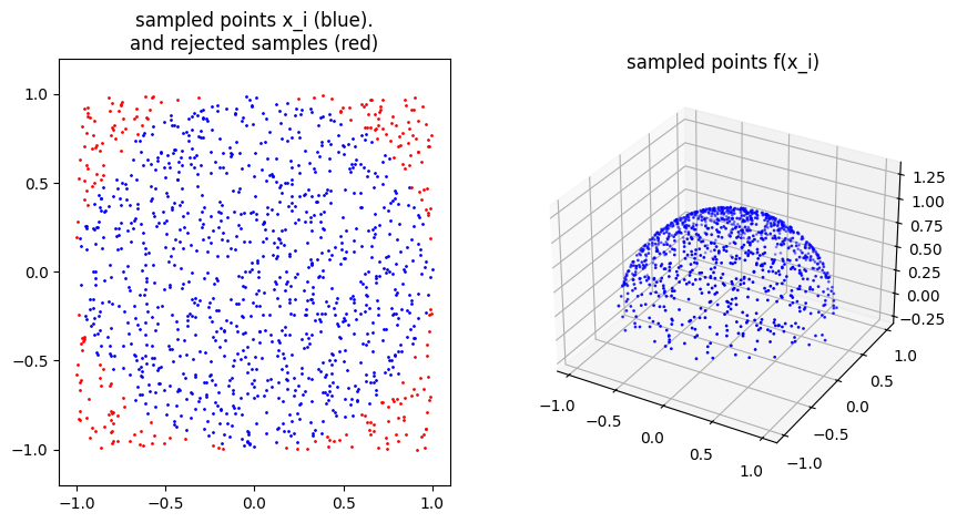
Below, we see a solution to compute the volume of the (half-) sphere. Here, $\Omega=\{x,y\in \mathbb{R}:x^2+y^2\leq 1\}$ with known volume (area) of $A=\pi$ and $f(x,y)=\sqrt{1-x^2-y^2}$ . To sample the uniformly distributed points in the circle we use rejection sampling, i.e. we draw $x,y$ independent uniformly in $[-1,1]^2$ and accept the point if $x^2-y^2\leq 1$ .

points_in = [list(),list()] #collect data on points sampled inside the circle
points_out = [list(),list()] #collect data on points sampled outside the circle
spherepoints = [list(),list(),list()] #collect data on points on the sphere

def sample_in_circle(radius:float=1.0) -> tuple[float,float]:
    """
    Uses rejection sampling to gerate a uniformly dusributed point in a circle with given radius
    :param radius: radius of the circle
    :return: x and y coordinate of a random point inside the circle
    """
    rsq = radius**2 #compute this upfron saves a little time
    while True:
        x = radius*(2.0*np.random.random()-1.0) # 2*X-1 transforms a U(0,1) to a U(-1,1)
        y = radius*(2.0*np.random.random()-1.0)
        if x**2+y**2<=rsq:
            points_in[0].append(x)
            points_in[1].append(y)
            return x,y
        else:
            points_out[0].append(x)
            points_out[1].append(y)

def mc_integration_circle(fun:Callable[[float,float],float],mc_samples:int,radius:float=1.0) -> float:
    """
    Integrates a function fun over a circular integration area with given radius using Monte Carlo integration
    :param fun: scalar function with two inputs x,y
    :param mc_samples: number of monte carlo samples
    :param radius: radius of the circle
    :return: numerically computed integral over the circle
    """
    xs = [sample_in_circle(radius) for i in range(mc_samples)]
    x_vec = [fun(*x) for x in xs]
    spherepoints[0] = [x[0] for x in xs]
    spherepoints[1] = [x[1] for x in xs]
    spherepoints[2] = x_vec
    B = np.pi*radius**2
    return B*sum(x_vec)/mc_samples

np.random.seed(12345) # make experiments reproducible
radius = 1.0
fun = lambda x,y:(radius**2-x**2-y**2)**0.5 # from x^2+y^2+z^2=radius^2
sphere_vol_anal = 4/3*np.pi*radius**3 # analytic volume
sphere_vol_mc = 2*mc_integration_circle(fun,1000,radius)
print(f'volume of sphere, analytic: {sphere_vol_anal}')
print(f'volume of sphere, monte carlo: {sphere_vol_mc}')
plt.figure(figsize=(10,5))
plt.subplot(1,2,1)
plt.scatter(points_in[0],points_in[1],s=1,c='b')
plt.scatter(points_out[0],points_out[1],s=1,c='r')
plt.title('sampled points x_i (blue).\nand rejected samples (red)')
plt.axis('equal')
plt.subplot(1,2,2,projection='3d')
plt.gca().scatter(spherepoints[0], spherepoints[1],spherepoints[2], c='b', s=1)
plt.title('sampled points f(x_i)')
plt.axis('equal')
plt.show()

volume of sphere, analytic: 4.1887902047863905
volume of sphere, monte carlo: 4.167871355208635

Monte Carlo Simulation¶

Next to Monte Carlo Integration and stochastic optimisation (e.g. genetic algorithms or simulated annealing, see Chapter Parameter Calibration), which is often classified as a Monte Carlo method due to the use of stochasticity, so-called Monte Carlo (MC) Simulation is another very important application of the method. In this process, a simulation model is used to generate the samples, whereby either the simulation model itself is stochastic, the parameters or inputs are varied stochastically, or both. One evaluation of the model as part of a MC simulation is called one (simulation) run.

Because every individual run is itself stochastic, the overall MC simulation is as well. Therefore, the key to a successful and reproducible MC Simulation lies in the configuration of the corresponding random number generator(s). The strategy depicted in Figure 1, where every simulation run is explicitly assigned a unique random number seed (see Chapter Pseudo Random Number Generation for details) is “cleanest” way to make the experiment repeoducible. Hereby, the individual seeds should initialise individual random number streams used solely within the corresponding simulation run. While specifying a single seed for a global pseudo random number generator at the start of the MC simulation is in principle sufficient, the strategy becomes unhandy when the user wants to reproduce selected individual runs or use multithreading/processing to compute individual runs in parallel.

Figure 1:Classic setup of a Monte Carlo Simulation using individual seeds for the individual runs.

The final result of the MC simulation is a list of simulation results. As before we will call them $x_1,\dots,x_M$ and consider them to be i.i.d. observations of a random variable $X\sim D$ . In order to understand $X$ and the underlying distribution $D$ , we perform statistics on the sample. The most prominent ones are the sample mean

\mathbb{E}(X)=\mu\approx\overline{X}_M=\frac{1}{M}\sum_{i=1}^{M}x_i,

(11)

and the sample variance

\mathbb{V}(X)=\mathbb{E}((X-\mu)^2)=\sigma^2\approx\overline{s}^2_M=\frac{1}{M-1}\sum_{i=1}^{M}\left(x_i-\overline{X}_M\right)^2.

(12)

Note that the factor $1/(M-1)$ instead of $1/M$ is used to make the estimator free of bias (i.e. that $\mathbb{E}(s_M^2)=\sigma^2$ ) and distinguishes the sample from the empirical variance.

Since the samples are simulation results, it is important to understand, that the individual observations may be scalars, but are more likely to be vectors or (vector-valued-) time series. This must be considered when computing statistics.

Case-Study: Multiple Server Queue¶

We will utilse the implemented model from Case-Study: Multiple Server Queue which is a classic discrete event simulation modelling the behaviour of a queue in front of a server, e.g. a supermarket queue. The model uses average values for arrival and service time as parameters and returns a time-series of queue lengths. We refer to the corresponding chapter for details and background of the model - for now all that matters is that it requires two scalar parameters and returns a non-equidistant time-series of integer values.

In particular the last part makes computation of statistics more complicated since all individual time-series have different event-times. One solution to this would be to define a common vector of evaluation times.

k = 2
mu_a = 1
mu_s = 2
tend = 1000

def monte_carlo_run(seed:int) -> tuple[np.ndarray,np.ndarray]:
    """Wrapper for a single monte carlo run
    :return: list of times and correspondin queue lengths
    """
    des = DESSimulator()  # create a DES simulator class
    msq = MultipleServerQueue(
        des, seed, k, mu_a, mu_s
    )  # create MSQ instance
    msq.sim.add(RunEvent(), 0)  # add the Run event
    return msq.run(tend) # run the model

mc_samples = 100 # number of samples
results = list()
for i in range(mc_samples):
    results.append(monte_carlo_run(i)) # seed = list index

def interp_des(t:np.ndarray,x:np.ndarray,tev:np.ndarray) -> np.ndarray:
    """
    Interpolates the timeseries x with event times t using a zero-order hold.
    Evaluates at the points tev
    :param t: event times
    :param x: values at the events
    :param tev: evaluation times
    :return: values at the evaluation times
    """
    f = interp1d(t,x,kind="previous")
    return f(tev)

# visualise the results
plt.figure(figsize=(10,5))
for t,x in results:
    plt.step(t,x,color='k',linewidth=0.5)
# compue mean
tev = np.arange(0,tend)
res = [interp_des(t,x,tev) for t,x in results]
mean = sum(res)/len(res)
plt.plot(tev,mean,color='r') # step plot does not make sense anymore
plt.show()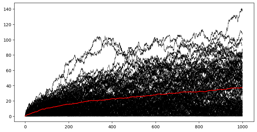

How many Monte Carlo Runs?¶

It is clear, that the number of samples $M$ is a relevant measure for how well the underlying distribution can be understood. The higher $M$ , the more robust are the statistics and therefore also distribution and moment estimates. Unfortunately, the number of samples that can be calculated is directly linked to the computing time required. This is a particularly significant limiting factor in the case of microscopic models, such as agent-based models, which are known to be computationally demanding itself. So one need methods to be able to make a sound estimate as to how many runs are minially required to achieve robust statements. Although the corresponding problem is a sole mathematical one, there is suprisingly no single best technique for this. We illustrate some concepts:

Surprisingly, the literature contains a large number of simulation studies in which the number of MC simulations carried out is not properly justified. Often, a more or less arbitrary power of 10 is chosen maybe as a result of computational time constraints, without actually studying the properties of the distribution or the convergence behaviour of the MC simulation. Of course, that is not a good solution, because the number of samples should depend primarily on the distribution characteristics and the desired accuracy of the statistics.

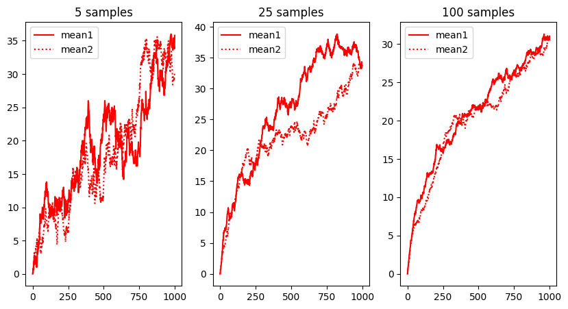
V2: Stability of Results¶

A simple and common approach is to check the statistics derived from the samples for stability. This involves repeating the MC experiment several times (using different random number generator seeds) and analysing the results statistically. If the resulting statistics are sufficiently close to one another, the number of MC samples is sufficient to produce statistics that are largely free from fluctuation.

Case-Study: Multiple Server Queue - Stability of Results¶

Below we execute the MC simulation twice and compare the sample means. Observe how the two sample means differ for different number of MC samples.

np.random.seed(12345)
plt.figure(figsize=(10,5))
for ind,mc_samples in enumerate([5,25,100]):
    results = list()
    for i in range(mc_samples):
        results.append(monte_carlo_run(np.random.randint(0,10000))) #seed the run with a top-level rng
    res = [interp_des(t,x,tev) for t,x in results]
    mean1 = sum(res)/len(res)
    results = list()
    for i in range(mc_samples):
        results.append(monte_carlo_run(np.random.randint(0,10000))) #seed the run with a top-level rng
    res = [interp_des(t,x,tev) for t,x in results]
    mean2 = sum(res)/len(res)
    plt.subplot(1,3,ind+1)
    plt.plot(tev,mean1,color='r',linestyle='-',label='mean1')
    plt.plot(tev,mean2,color='r',linestyle='dotted',label='mean2')
    plt.legend()
    plt.title(f'{mc_samples} samples')
plt.show()

V3: Stopping Rule - Static¶

The most sophisticated approach to estimate the number of required samples upfront is the use of a stopping rule. This method is usually applied to estimate the number of samples required to accurately estimate a scalar mean value $\mu\in \mathbb{R}$ by the sample mean $\overline{X}_M$ , with the right mathematics the concept can be extended to other moments and non-scalar outcomes as well Bicher et al. (2022).

The foundation to the stopping rule concept lies in the probabilistic accuracy statement

P(|\overline{X}_M-\mu|>\delta)<p,

(13)

whereas we quantify the likelihood $p$ that the sample mean $\overline{X}_M$ of $M$ runs is farther away from the actual unknown mean $\mu$ than $\delta$ . The idea of a stopping rule is to quantify a relation between $p,\delta$ and $M$ . Interestingly, as illustrated in Bicher et al. (2022), there are multiple approaches to do so.

The most applicable of them is the Gaussian approach which follows from the central limit theorem (see e.g. ()[doi:10.1007/978-0-387-87857-7]): For an arbitrary random number $X$ with finite mean $\mu$ and standard deviation $\sigma$ , we find

\sqrt{M}\frac{\overline{X}_M-\mu}{\sigma}\underset{M\rightarrow \infty}{\longrightarrow} Z\sim \mathcal{N}_{0,1}.

(14)

That means, the statement to the left converges, in distribution, towards a standard normally distributed random number. As a result, we may estimate that $\sqrt{M}\frac{\overline{X}_M-\mu}{\sigma}\sim \mathcal{N}_{0,1}$ for sufficiently large $M$ and use the quantiles of the normal distribution to quantify probabilities:

P\left(\sqrt{M}\frac{\overline{X}_M-\mu}{\sigma}>x\right)\approx P\left(\sqrt{M}\frac{\overline{X}_M-\mu}{\sigma}<-x\right)\approx \Phi(-x).

(15)

Hereby $\Phi$ stands for the cumulative distribution function of the normal distribution

\Phi(x)=\int_{-\infty}^{x}\frac{1}{\sqrt{2\pi}}e^{-t^2/2}dt.

(16)

That means, setting $\delta=x\frac{\sigma}{\sqrt{M}}$ , we find

p>P(|\overline{X}_M-\mu|>\delta)=P(\overline{X}_M-\mu<-\delta)+P(\overline{X}_M-\mu>\delta)

(17)

=P\left(\sqrt{M}\frac{\overline{X}_M-\mu}{\sigma}<x\right)+P\left(\sqrt{M}\frac{\overline{X}_M-\mu}{\sigma}>x\right)\approx 2\Phi(-x)=2\Phi\left(-\frac{\delta\sqrt{M}}{\sigma}\right).

(18)

Solving this inequality w.r. to $M$ leads $M>\frac{\sigma^2}{\delta^2}\left(\Phi^{-1}\left(\frac{p}{2}\right)\right)^2$ . We see, that higher variance $\sigma^2$ , smaller tolerance $\delta$ and smaller acceptance propbability $p$ influence the number of required iterations.

As soon as one has a proper estimate (upper bound) for the variance, we can compute the minimum required Monte Carlo samples to estimate the mean value with the given accuracy. A variance estimate can be carried out by an initial Monte Carlo simulation and computing the sample variance $s_M^2$ .

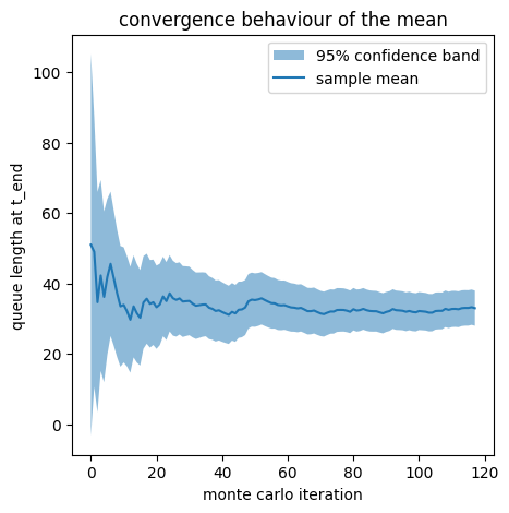
Another possible application of the formula is that we can derive a confidence band for a given number of samples $M$ and confidence level $100\cdot (1-p)\%$ . Then,

\left[\overline{X}_M+\Phi^{-1}\left(p/2\right)\frac{\sigma}{\sqrt{M}},\overline{X}_M-\Phi^{-1}\left(p/2\right)\frac{\sigma}{\sqrt{M}}\right],

(19)

is a $100\cdot (1-p)\%$ confidence interval for the real mean $\mu$ . This statement can also be used to reason a certain number of Monte Carlo samples.

Case-Study: Multiple Server Queue - Stopping Rule¶

To simplify the case study to a scalar problem, we will only investigate the state of the length of the queue at the simulation end time $t_{end}$ instead of the full timeseries.

delta = 5 # absolute bound
p = 0.05 # failure likelihood
mc_samples_init = 10 # initial sample size to estimate the variance

np.random.seed(12345)

# compute initial monte carlo samples for variance
results = list()
for i in range(mc_samples_init):
    t,x = monte_carlo_run(np.random.randint(0,10000))
    results.append(x[-1])

sample_variance = np.var(results) # compute sample variance
mc_samples = int(np.ceil(sample_variance/delta**2*scipy.stats.norm.ppf(p/2)**2)) # ppf = Phi^-1
print(f'required iterations ac. to formula: {mc_samples}')

# cotinue monte carlo simulation until the required iteration count
if mc_samples>mc_samples_init:
    for i in range(mc_samples-mc_samples_init): #continue sampling
        t,x = monte_carlo_run(np.random.randint(0,10000))
        results.append(x[-1])

# inverse application: evaluate confidence intervals for given M and p for plotting
deltas = np.array([-scipy.stats.norm.ppf(p/2)*sample_variance**0.5/(i+1)**0.5 for i in range(mc_samples)])
sample_means = np.array([np.average(results[:i+1]) for i in range(mc_samples)])
plt.figure(figsize=(5,5))
plt.fill_between(list(range(mc_samples)),sample_means-deltas,sample_means+deltas,label=f'{100*(1-p):.0f}% confidence band',alpha=0.5)
plt.plot(sample_means,label='sample mean')
plt.legend()
plt.xlabel('monte carlo iteration')
plt.ylabel('queue length at t_end')
plt.title('convergence behaviour of the mean')
plt.show()

required iterations ac. to formula: 118

Although this Normal distribution -inspired concept is well applicable and leads to reasonable sample sizes, it is only an asymptotic rule, since $\sqrt{M}\frac{\overline{X}_M-\mu}{\sigma}\sim \mathcal{N}_{0,1}$ and $\sqrt{s_M^2}\approx \sigma$ are only approximations. There are plenty and much more complex approaches to work around this problem. The mathematic foundation to derive these formulas is the field of so-called concentration inequalities.

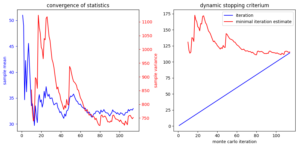
V4: Stopping Rule - Dynamic¶

In the example before, the initial Monte Carlo simulation for estimation of the sample variance was performed independent of the actual Monte Carlo simulation. Clearly there is no need to disentangle the two and update the variance and mean value estimate dynamically. This way, the variance estimate and consequently the minimal-sample estimate becomes continuously more accurate, and we may dynamically stop the loop as soon as the iteration index is larger or equal to the sample estimate.

Dynamic Moment Update¶

To carry out this process as efficiently as possible, it is practicable to update the estimators for the moments (i.e. mean and variance) dynamically, i.e. so that it is not necessary to iterate through all previously calculated results in every Monte Carlo loop. For example, the following iteration is obtained from the formula for the sample mean

\overline{X}_M=\frac{1}{M}\sum_{i=1}^{M}x_i=\frac{1}{M}\left(x_M+\frac{M-1}{M-1}\sum_{i=1}^{M-1}x_i\right)=\frac{1}{M}\left(x_M+(M-1)\overline{x}_{M-1}\right)=\frac{1}{M}x_M+\frac{M-1}{M}\overline{X}_{M-1}.

(20)

Therefore, we may compute the new sample mean $\overline{X}_M$ from the old one $\overline{X}_{M-1}$ and the new sample $x_m$ . For the standard deviation / variance the startegy is less straight forward but still possible. We may exploit a feature related to the Steiner-Identity $V(X)=E(X^2)-E(X)^2$ : Consider the sample mean for the squares, i.e. $\overline{X^2}_M=\frac{1}{M}\sum_{i=1}^{M}x^2_i$ , for which we find the analogous dynamic update

\overline{X^2}_M=\frac{1}{M}x^2_M+\frac{M-1}{M}\overline{X^2}_{M-1},

(21)

then

s^2_M=\frac{M}{M-1}\left(\overline{X^2}_M-\overline{X}_M^2\right).

(22)

Note that the factor $\frac{M}{M-1}$ is used to compute the sample variance from the empirical variance.

delta = 5 # absolute bound
p = 0.05 # failure likelihood
mc_samples_init = 10 # initial threshold until the variance estimate can be used
mc_samples_upper_bound = 100000 # upper bound for how many sample we can make

np.random.seed(12345)

results = list()
sample_mean = 0 # initialise sample mean
sample_mean_squares = 0 # initialise sample mean of squares

# for plot
iterations = list()
iterations_min = list()
sample_means = list()
sample_variances = list()

for i in range(1,mc_samples_upper_bound+1): # shift by 1 to make update formulas easier to compute
    t,x = monte_carlo_run(np.random.randint(0,10000))
    results.append(x[-1])
    sample_mean = 1/i*x[-1]+(i-1)/i*sample_mean # dynamic moment update (sample mean)
    sample_mean_squares = 1/i*x[-1]**2+(i-1)/i*sample_mean_squares # dynamic moment update (sample mean of squares)
    if i>=mc_samples_init:
        sample_variance = i/(i-1)*(sample_mean_squares-sample_mean**2) # compute sample variance
        i_min = sample_variance/delta**2*scipy.stats.norm.ppf(p/2)**2 # evaluate minimal iterations with formula
        if i_min<=i: # break if current iteration is larger or equal to minimal iterations from formula
            print(f'dynamically stopped after iteration {i}')
            break
    else:
        i_min = None
        sample_variance = None
    ## for plotting
    iterations.append(i)
    iterations_min.append(i_min)
    sample_means.append(sample_mean)
    sample_variances.append(sample_variance)
plt.figure(figsize=(10,5))
plt.subplot(1,2,1)
plt.plot(iterations,sample_means,color='b',label='sample mean')
plt.ylabel('sample mean')
plt.gca().yaxis.label.set_color('b')
plt.gca().tick_params(axis='y', colors='b')
plt.twinx()
plt.plot(iterations,sample_variances,color='r',label='sample variance')
plt.ylabel('sample variance')
plt.gca().yaxis.label.set_color('r')
plt.gca().tick_params(axis='y', colors='r')
plt.xlabel('monte carlo iteration')
plt.title('convergence of statistics')
plt.subplot(1,2,2)
plt.plot(iterations,iterations,color='b',label='iteration')
plt.plot(iterations,iterations_min,color='r',label='minimal iteration estimate')
plt.legend()
plt.xlabel('monte carlo iteration')
plt.title('dynamic stopping criterium')
plt.tight_layout()
plt.show()

dynamically stopped after iteration 115

References¶

Dekking, F. M., Kraaikamp, C., Lopuhaä, H. P., & Meester, L. E. (2005). A Modern Introduction to Probability and Statistics: Understanding why and how (Vol. 488). Springer.
Metropolis, N. (1987). The Beginning of the Monte Carlo Method. Los Alamos Science, Special Issue 1987, 125–130.
Daudin, F. M. (1801). Histoire naturelle, générale et particulière des reptiles; ouvrage faisant suite a l’Histoire naturelle générale et particulière, composée par Leclerc de Buffon, et rédigée par CS Sonnini... par FM Daudin... tome premier-huitième (Vol. 1). de l’imp. de F. Dufart.
Behrends, E. (2024). Buffon: Hat er Stöckchen geworfen oder hat er nicht? In Pi und Co. Kaleidoskop der Mathematik (pp. 173–175). Springer.
Bicher, M., Wastian, M., Brunmeir, D., & Popper, N. (2022). Review on Monte Carlo Simulation Stopping Rules: How Many Samples Are Really Enough? SNE Simulation Notes Europe, 32(1), 1–8. 10.11128/sne.32.on.10591