
In this chapter we discuss concepts for parameter calibration.
Objectives:
What does “calibration” mean?
How do we define error metrics between simulation and reference data?
Which algorithms exists to minimize this error?
from abc import abstractmethod
from collections.abc import Callable
from typing import Self

import numpy as np
from matplotlib import pyplot as plt
from scipy import spatial
from scipy.integrate import solve_ivp
from scipy.optimize import minimize
from scipy.stats import qmc
Calibration - Basic Idea
The term calibration refers to the systematic determination of parameter values for given reference solutions. We may introduce this formally, by considering the implemented model as a mapping which maps input and parameters onto output , as shown in the figure below.

The calibration problem is then formulated by finding when and are given, i.e. to find s.t. . The corresponding input is called the calibration scenario and is usually referred to a calibration reference and is usually given by data. In the ideal case, would be given analytically so it can be inverted, however for usual modelling and simulation applications this is not the case, meaning that we need to determine
with other means, whereas refers for an error metric between simulation result and reference outcome . An optimisation problem results, meaning that any algorithm used for numerical optimisation can also be applied for calibration.
As seen in the problem statement, not only the computerised model but also the error metric define the found optimum. Therefore it must be chosen with equal care.
In practice, is usually a vector (parameter vector) and is not calibrated as a whole, meaning, it can be split into two sub-vectors: . Here, denotes the vector of those parameters that are parameterised directly from data, estimates or other sources of information (bound parameters). The vector denotes the vector of free parameters, which are ultimately determined via calibration.
Rule of thumb states that the dimension of the fitted parameter vector must be equal or smaller than the amount of reference information available. However, it requires a lot of experience and system knowledge to extimate if this is the case. As a trivial example, a scalar reference value will not be enough to fit a three-dimensional parameter vector. A whole reference time-serie might, but not always. Suppose the model is defined by , there will nevere be a way to determine correct distinct values for and from the reference output of the model alone. Anyhow, clearly, the more reference scenario/data pairs are available, the better the model can be fitted. In the optimal case, a proper distinction between training- and test-data should be envisioned.
It should be noted that parameter calibration, as a part of the parameter identification process, has various names including model fitting or model training. However, in particular the latter one is usually applied in case of black-box approaches like regression.
Example: Lithium Cluster Dynamics
Background
This case-study was the first of more than 20 defined benchmarks of the Austrian and German Arbeitsgemeinschaft Simulation (ARGESIM) published 1991 in the journal Simulation News Europe Husinsky (1991). It’s original purpose was the testing and comparison of simulation evironments for how they could handle the corresponding nonlinear and stiff differential equation model. Here we use it as a case study for parameter calibration.
System and Problem Statement
We investigate the bombardment of a lithium crystal with electrons. When electrons hit the surface with sufficient energy, so-called -centres are formed in the crystal. An F-center, FARBE center (from the original German Farbzentrum), is a type of crystallographic defect in which an anionic vacancy in a crystal is filled by one or more unpaired electrons. The origin electrons in such a vacancy tend to absorb light in the visible spectrum such that a material that is usually transparent becomes coloured. Those centres can either immediately cause desorption of a lithium atom, or they agglomerate near the surface of the material and form aggregates of various sizes, called -centres. These centres break down after a characteristic time into - centres again as their state is physically unstable. Conventionally -centres are called -centres and -centres will be denoted as -centres. The purpose of the model is to correctly depict/forecast the concentration of and centres under electron bombardment.

Conceptual Model
The dynamic of the lithium clusters can either directly be modelled via ordinary differential equations or using a System Dynamics approach (which eventually leads to the same model equations). Here is a picture of the stock and flow diagram:

The stocks and denote the total concentration of F-,M-,R- centres inside the Lithium crystal. Flows between the stocks describe either decay of larger centres into smaller or fusion of smaller ones into larger. The external flow into is the production of new -centres via bombardment (irradiation). The corresponding auxiliary function is equal to until is reached and 0 thereafter. The external flow from is the emission of -centres from the crystal. The underlying differential equations are
The parameters in these equations cab be understood as follows: Parameters and denote the rate how fast - and - centres collapse to either two -centres, or one - and one - centre, respectively. The growth rates and denote how fast lower order centres form higher order centres. Parameter stands for the rate how fast -centres evaporate at the surface of the crystal.
As said, we model as temporarily constant over the interval and 0 otherwise. We can write this as the difference between two heavyside functions:
Note, that the system can easily be extended taking into account formation of larger aggregates ( centres), but this is not the goal of the case study in this section.
Model Parameters
The model can be seen to have 10 parameters, nine of which have been assigned defalut values in the original publication Husinsky (1991). These are:
| Parameter | Symbol | Default Value | Parameter Space |
|---|---|---|---|
| Rate for fusion of one - and one -centre into new -centres | 1 | ||
| Rate for fusion of two -centres into new -centres | 0.1 | ||
| Rate of decay of -centres into one - and one -centre | 0.1 | ||
| Rate of decay of -centres into two -centres | 1 | ||
| Rate of decay of -centres | 1000 | ||
| Creation rate of new -centres by bombardment | 10000 | ||
| End of bombardment | 10 | ||
| Initical concentration of -centres | 9.975 | ||
| Initical concentration of -centres | 1.674 | ||
| Initical concentration of -centres | 84.99 |
Implemented Model
The model is implemented using the solve_ivp method provided by SciPy using the BDF solver (instead of the standard RK45) because the ODE system is stiff.
class LithiumClusterConfig:
    def __init__(self) -> None:
        """Class for configuring a LithiumClusterModel
        :return:
        """
        self.kr: float = 0.0
        self.kf: float = 0.0
        self.dr: float = 0.0
        self.dm: float = 0.0
        self.lf: float = 0.0
        self.pc: float = 0.0
        self.tstop: float = 0.0
        self.f0 = 0.0
        self.m0 = 0.0
        self.r0 = 0.0

    def from_array(self, params: np.ndarray) -> None:
        """Initialises the configuration with a specific parameter and input selection
        :params: list or array containing the parameter/input values
        :return:
        """
        if np.any(params) < 0:
            print("values smaller than zero detected..truncating")
            params = np.array([max(p, 0) for p in params])
        self.kr: float = params[0]
        self.kf: float = params[1]
        self.dr: float = params[2]
        self.dm: float = params[3]
        self.lf: float = params[4]
        self.pc: float = params[5]
        self.tstop: float = params[6]
        self.f0: float = params[7]
        self.m0: float = params[8]
        self.r0: float = params[9]

    def to_array(self) -> np.ndarray:
        """Converts the configuration object to an array
        :return:
        """
        return np.array(
            [
                self.kr,
                self.kf,
                self.dr,
                self.dm,
                self.lf,
                self.pc,
                self.tstop,
                self.f0,
                self.m0,
                self.r0,
            ]
        )

    def copy(self) -> Self:
        """Deep copy of the configuration object
        :return: copy
        """
        s = LithiumClusterConfig()
        s.from_array(self.to_array())
        return s

    def __str__(self) -> str:
        """String representation
        :return: a summary of the model parameters
        """
        return ",".join(["{:6s}".format(f"{x:.02f}") for x in self.to_array()])


class LithiumClusterModel(LithiumClusterConfig):
    def __init__(self, config: LithiumClusterConfig) -> None:
        """Initialises the model with a specific parameter selection
        :param config: instance of the configuration object
        :return:
        """
        super().__init__()
        self.from_array(config.to_array())

    def p(self, t) -> float:
        """Bombardment function
        :param t: current time
        :return: current bombardment impact
        """
        return self.pc if t <= self.tstop else 0.0

    def rhs(self, t: float, x: np.ndarray) -> np.ndarray:
        """Right hand side of the ODE model
        :param t: t
        :param x: x
        :return: dx/dt
        """
        p = self.p(t)
        f = x[0]
        m = x[1]
        r = x[2]
        df = (
            p
            - self.lf * f
            - 2 * self.kf * f**2
            - self.kr * f * m
            + 2 * self.dm * m
            + self.dr * r
        )
        dm = self.kf * f**2 - self.kr * f * m - self.dm * m + self.dr * r
        dr = self.kr * f * m - self.dr * r
        return np.array([df, dm, dr])

    def run(self, tend: float) -> tuple[np.ndarray, np.ndarray]:
        """Executes the model over a certain timespan
        :param tend: simulation time-span
        :return: array with time values, 2d array with F-,M-,R- center concentration values
        """
        y0 = np.array([self.f0, self.m0, self.r0])
        sol = solve_ivp(self.rhs, y0=y0, t_span=[0, tend], method="BDF")
        return sol.t, sol.y
# simple evaluatuon with default parameters
default_params = LithiumClusterConfig()
default_params.kr = 1.0
default_params.kf = 0.1
default_params.lf = 1000.0
default_params.dr = 0.1
default_params.dm = 1.0
default_params.pc = 10000.0
default_params.tstop = 10.0
default_params.f0 = 9.975
default_params.m0 = 1.674
default_params.r0 = 84.99
model = LithiumClusterModel(default_params)
T, X = model.run(20)
plt.figure(figsize=(8, 4))
plt.plot(T, X[0, :], label="f(t)")
plt.plot(T, X[1, :], label="m(t)")
plt.plot(T, X[2, :], label="r(t)")
plt.legend()
plt.show()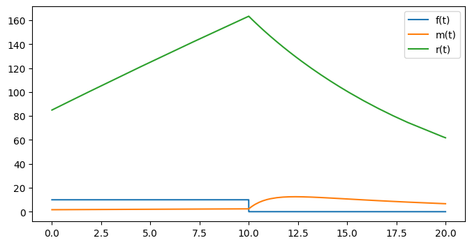
# parameter variation for lf
plt.figure(figsize=(8, 4))
for lf in [10 ** ((5 + i) / 3) for i in range(1, 8)]:
    params = default_params.copy()
    params.lf = lf
    model = LithiumClusterModel(params)
    T, X = model.run(10)
    plt.plot(T, X[0, :], label=f"f(t;{lf:.0f})")
plt.gca().set_yscale("log")
plt.gca().set_xscale("log")
plt.legend()
plt.show()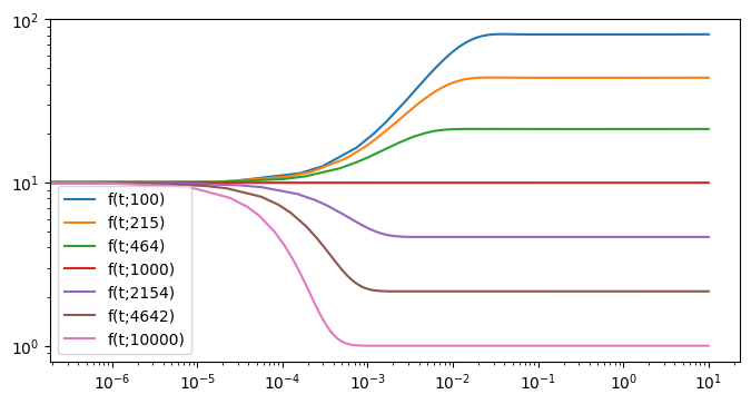
Example: Lithium Cluster Dynamics ((Synthetic) Reference Data)
To investigate different methods for calibration we first require reference data to fit the model to.
Considering that we do not have real measurements available, we will create the data synthetically using the model itself. This has the additional benefit that the parameter values for the optimal fit are a-priori known.
In this case study, we will use the default parametrisation / input to generate the reference for an observation period of . We will evaulate the reference at 200 randomly selected points in time and add a normally distributed noise.
n_data = 200
np.random.seed(12345)  # fix the seed to be redproducible
model = LithiumClusterModel(default_params)
t_end = 20.0
t_sol, y_sol = model.run(t_end)  # execute the model with the default parameters
# create a random time-base with n_data points
t_ref = t_end * np.random.random(n_data)
t_ref.sort()
# interpolate the sim-result and add noise
y_ref = np.zeros([3, n_data])
y_ref[0, :] = np.interp(t_ref, t_sol, y_sol[0, :]) + 0.5 * np.random.randn(n_data)
y_ref[1, :] = np.interp(t_ref, t_sol, y_sol[1, :]) + 0.5 * np.random.randn(n_data)
y_ref[2, :] = np.interp(t_ref, t_sol, y_sol[2, :]) + 2 * np.random.randn(n_data)
# compare sim-result with synthetic data
plt.figure(figsize=(12, 5))
for i, lbl in enumerate(["f(t)", "m(t)", "r(t)"]):
    plt.subplot(1, 3, i + 1)
    plt.plot(t_sol, y_sol[i, :], "k", label="sim_result")
    plt.plot(t_ref, y_ref[i, :], "ob", label="synthetic data")
    plt.legend()
    plt.title(lbl)
plt.show()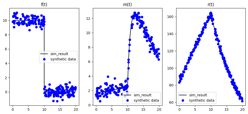
Case Study: Lithium Cluster Dynamics - Error Function
In order to apply calibration metaheuristics it is relevant to define error metrics as objetive function for the optimisation. For the state example we will use the sum of the element-wise mean square error (MSE) for all three curves , spline-interpolated on the 100-element time vector .
To investigate how well the simulation could fit the data, we compute the error function for the simulation results with the default setup, i.e. the one which was already used to compute the data.
def error_lithium_cluster(t_sim: np.ndarray, y_sim: np.ndarray) -> float:
    """Computes the error between the simulation results and the reference data
    :param t_sim: vector with time-values for the simulation result
    :param y_sim: matrix with f,m,r curves for the simulation result
    :return: error between simulation and reference data
    """
    t_cmp = np.arange(0, 20, 0.2)
    err = [0, 0, 0]
    for i in range(3):
        y_ref_cmp = np.interp(t_cmp, t_ref, y_ref[i, :])
        y_ref_sim = np.interp(t_cmp, t_sim, y_sim[i, :])
        err[i] = ((y_ref_cmp - y_ref_sim) * (y_ref_cmp - y_ref_sim)).sum() / 100.0
    return sum(err)


model = LithiumClusterModel(
    default_params
)  # execute the model with the default parameters
t_end = 20.0
t_sol, y_sol = model.run(t_end)
print(f"Reference error: {error_lithium_cluster(t_sol, y_sol)}")
Reference error: 3.0800062730246367
Case Study: Lithium Cluster Dynamics - Free Parameters
For calibration we split the ten-element parameter-vector from LithiumClusterConfig into two sub-vectors: the first one contains all parameters with a-prior known values, e.g. because we found or computed them directly from data. The second one, henceforth referred to as , contains all free parameters which are subject to calibration. Of those values, we assume to know their space of feasible values .
full_parameter_space = np.array(
    [
        [0.2, 3.0],
        [0.05, 0.2],
        [0.01, 0.2],
        [0.3, 3.0],
        [100.0, 10000.0],
        [2000.0, 20000.0],
        [5.0, 20.0],
        [0.0, 10.0],
        [0.0, 100.0],
        [0.0, 20.0],
    ]
)  # all boundaries of all paramaters


def extract_free_parameters(
    free_parameter_indices: np.array, full_parameter_vector: np.array
) -> np.array:
    """Method to extract the subvector of free parameters from a full parameter vector
    :param free_parameter_indices: indices to free parameters
    :param full_parameter_vector: full parameter vector
    :return: subvector containing the free parameter values
    """
    return full_parameter_vector[free_parameter_indices]


def extract_free_parameter_space(free_parameter_indices: np.array):
    """Returns the parameter space to the free parameters
    :param free_parameter_indices: indices to free parameters
    :return: space for the free parameters
    """
    return full_parameter_space[free_parameter_indices, :]


def embed_free_parameters(
    free_parameter_indices: np.array, free_parameter_vector: np.array
) -> np.array:
    """Embeds the vector of free parameters into a vector of full parameters assuming that all other parameter values are known from the default parametrisation
    :param free_parameter_indices: indices to free parameters
    :param free_parameter_vector: vector with free parameter values
    :return: full vector with embedded values
    """
    arr = default_params.to_array()
    arr[free_parameter_indices] = free_parameter_vector
    return arr
The goal of the calibration is to minimize over the parameter-space with respect to whereas is interpreted as the simulation results associated with the free-parameter vector . To make this explicit, we wrap both into an LithiumClusterIndividual class which extends the LithiumClusterConfig. Its method map_to_parameterspace can be used to force the individual into a legitimate region.
Gradient-Based Methods
The most common strategy for optimization is given by gradient based methods, (or simply gradient method) which are defined by an iteration starting with an initial parameter guess . The methods are defined by the iteration
whereas stands for (an estimate of) the gradient of w.r. to , i.e.
and is a positive (definite) stepsize. Inituitively, gradient methods simplify vector-values minimisation problems to iterative scalar searches along the line of the greatest descent, i.e. . Since the methods improve one parameterset iteratively, they can be counted to the trajectory-based approaches (in cotrast to population-based concepts). Hereby is often found by iterative line-search concepts, there are also direct methods.
Gradient Descent
The most famous of the gradient methods is likely the Gradient Descent method, where is a small well chosen positive constant. That means the algorithm seemingly has one hyperparameter to tune. However, considering that the target function is solely known as black-box, gradient-based methods require estimates for the corresponding gradients. This must be done e.g. by numerical differentiation, for example:
for some small . This makes the gradient method a quasi-gradient method and adds another hyperparameter to define properly.
| Hyperparameter | Symbol | Range/Space | Considerations |
|---|---|---|---|
| stepwidth of the algorithm | positive scalar | heavily dependent on the problem. Too small long computation time, too large algorithm diverges | |
| stepsize for estimation of the gradient | positive scalar | should be chosen as small as possible to make an accurate derivative estimate but as large as required to avoid rounding errors |
Newton method
The Newton (or Newton–Raphson) Method is a well known gradient-based method to find roots of equations for some smoot function . The iteration is defined by , where refers to the Jacobi matrix of . However, any root finding algorithm can be applied to minimise/maximise smooth functions as well by applying the algorithm on the gradient instead of the orginal function. In this case, the iteration becomes
In this case, the Jacobi matrix of translates to the hessian matrix of evaluated at defined by
That means, the algorithm uses . Analogous to the Gradient Descent, the Newton method usually requires numerical estimates not only for gradient but also for the Hessian, e.g. by
This estimate is usually quite expensive to compute for every iterations, so that it is often avoided using simpler approximations, e.g. the Broyden-Fletcher-Goldberg-Shanno algorithm (Broyden, 1985) uses a “rank-1” approximation which only requires some vector computations with the gradient.
In general the Newton method does not use any hyperparameter, however in some situations the method must be damped to converge properly. This leads the Damped Newton Method
with some damping factor .
| Hyperparameter | Symbol | Range/Space | Considerations |
|---|---|---|---|
| damping factor | use smaller values only if does not leaad to convergence | ||
| stepsize for estimation of the gradient and hessian | positive scalar | should be chosen as small as possible to make an accurate derivative estimate but as large as required to avoid rounding errors |
We refer to standard literature about numerical optimization for more details, e.g. Numerical Optimization. Below the Gradient Descent and the damped Newton method is implemented and applied to a simple analytic case study with known minimum (the Booth-function, Jamil & Yang (2013)).
In the following, we will implement both methods and two base classes which they extend. These base classes will help us later to implement and test several other optimisation methods as well (i.e. more work now, less work later).
class Optimizer:
    def __init__(
        self, function: Callable[[np.ndarray], float] | None, name: str
    ) -> None:
        """Base class for optimization of methods
        :param function: function to minimize. Can be None to set it later on.
        :param name: name of the method
        """
        self.name = name
        if function == None:
            self.function_base = lambda x: 0
        else:
            self.function_base = function
        self.count = 0
        self.function_base = function
        self.p_sol = None
        self.err_sol = None

    def set_function(self, function: Callable[[np.ndarray], float]) -> None:
        """Can set the function also a-posteriori
        :param function: objective function to be minimized
        """
        self.function_base = function
        self.reset()

    def set_ground_truth(self, p_sol: np.ndarray) -> None:
        """Defines the reference solution to evaluate the performance of the method
        :param p_sol: reference parameter set
        """
        self.p_sol = p_sol
        self.err_sol = self.function_base(self.p_sol)

    def reset(self) -> None:
        """Resets the internal counter which tracks function evaluations"""
        self.count = 0

    def function(self, p: np.ndarray) -> float:
        """Applies the funtion to a given parameter vector and increments the counter
        :param p: parameter vector
        :return: value
        """
        self.count += 1
        return self.function_base(p)

    @abstractmethod
    def run(self, max_iter: int, p0: np.ndarray = None, color="r") -> np.ndarray:
        """Abstract run method.
        Performs some iteration until (at most) max_iter and uses, optionally, a starting value p0
        :param max_iter: maximum iterations
        :param p0: starting value
        :param color: optional color specification for plotting
        :return: optimized parameter vector
        """
        return np.array([])

    def stop(self) -> bool:
        """Override this method to specify a stopping criterium. Called after every update-step
        (Currently unused)
        :return: true, if the method should stop at this point
        """
        return False


class IterativeOptimizer(Optimizer):
    def __init__(
        self, function: Callable[[np.ndarray], float] | None, name: str
    ) -> None:
        """Wrapper class for every optimized which iteratively improves one parameter set at a time.
        :param function: function to minimize. Can be None to speficy later
        :param name: name of the method
        """
        super().__init__(function, name)

    def reset(self) -> None:
        """Resets all internal variables related to covergence tracking and output visualization"""
        super().reset()
        self.trajectory = list()
        self.fps = list()
        self.step = 0

    @abstractmethod
    def update_step(self, p: np.ndarray, fp: float) -> tuple[np.ndarray, float | None]:
        """Abstract method to performs an update step.
        :param p: current status of the iteration
        :param fp: function value at p
        :return: updated state and function value at this point. For the latter, return None, if it needs to be computed anew.
        """
        return np.array([]), None

    def print_msg(self) -> None:
        """Prints a message to analyze the convergence status at the current step
        :return:
        """
        if (
            len(self.fps) == 1 or self.fps[-1] != self.fps[-2]
        ):  # only print a message if we have some progress to show
            print(f"step {self.step}: {self.trajectory[-1]} -> {self.fps[-1]}")

    def print_final_msg(self) -> None:
        """Prints a summary message after the iteration
        :return:
        """
        if self.p_sol is not None:
            diff = self.trajectory[-1] - self.p_sol
            reldiff = diff / self.p_sol
            accx = np.linalg.norm(reldiff)
        else:
            accx = "undef."
        print(
            f"Summary: steps {self.step}, func-evals: {self.count}, accuracy x: {accx}, residual: {self.function_base(self.trajectory[-1])}"
        )

    def run(self, max_iter: int, p0: np.ndarray = None, color="r") -> np.ndarray:
        """Runs the iteration until (at most) max_iter (depending on the implementation of "stop").
        :param max_iter: maximum iterations
        :param p0: initial guess (must be given in this implementation!)
        :param color: color for plotting
        :return: optimized parameter set
        """
        assert p0 is not None, ValueError(
            "Iterative optimizer must have a p0 value which is not None"
        )
        self.reset()
        p = p0
        fp = self.function(p)
        self.trajectory.append(p)
        self.fps.append(fp)
        # print state for the initial condition
        self.print_msg()
        # start iteration
        for i in range(max_iter):
            self.step = i + 1
            p, fp = self.update_step(p, fp)
            self.trajectory.append(p)
            if fp == None:
                fp = self.function(p)
            self.fps.append(fp)
            self.print_msg()
            if self.stop():
                break
        # plot the trajectory
        # label for plot
        lbl = f"{self.name} (in {self.step} steps ({self.count} F-evals) from {self.fps[0]:.02f} to {self.fps[-1]:.02f})"
        n = len(self.trajectory)
        for i, (x0, x1) in enumerate(zip(self.trajectory[:-1], self.trajectory[1:])):
            plt.plot(
                [x0[0], x1[0]],
                [x0[1], x1[1]],
                color=color,
                alpha=(i + 1 + n / 5) / (n - 1 + n / 5),
                label=lbl if i == n - 2 else None,
            )
        self.print_final_msg()
        return self.trajectory[-1]


class NewtonOptimizer(IterativeOptimizer):
    def __init__(
        self,
        function: Callable[[np.ndarray], float] | None,
        h: float = 0.01,
        gamma: float = 0.5,
    ) -> None:
        """Implements the Newton method
        :param function: function to minimize. Can be None to specify later
        :param h: stepsize for estimation of the gradient
        :param gamma: stepsize for damped Newton step
        """
        super().__init__(function, name="newton")
        self.h = h
        self.gamma = gamma

    def update_step(self, p: np.ndarray, fp: float) -> tuple[np.ndarray, float | None]:
        """Performs a Newton step
        :param p: current status of the iteration
        :param fp: function value at p
        :return: updated state and corresponding function value (will be always None in this method)
        """
        dim = len(p)
        # compute gradient and hessian
        id = np.identity(dim)
        grad = np.zeros(dim)
        hess = np.zeros([dim, dim])
        fpi = list()
        # evaluate the error function at selected points in proximity
        for i in range(dim):
            fpi.append(self.function(p + self.h * id[:, i]))
        for i in range(dim):
            grad[i] = (fpi[i] - fp) / self.h  # compute the gradient
            for j in range(dim):
                fpij = self.function(p + self.h * id[:, i] + self.h * id[:, j])
                hess[i, j] = (
                    fpij - fpi[i] - fpi[j] + fp
                ) / self.h**2  # compute the hessian
        # use linear-solve instead of explicitly computing the inverse
        diff = np.linalg.solve(hess, self.gamma * grad)
        # update
        return p - diff, None


class GradientDescentOptimizer(IterativeOptimizer):
    def __init__(
        self,
        function: Callable[[np.ndarray], float] | None,
        h: float = 0.01,
        alpha: float = 0.1,
    ) -> None:
        """Implements the Gradient Descent method
        :param function: function to minimize. Can be None to specify later
        :param h: stepsize for estimation of the gradient
        :param alpha: stepsize for the descent step
        """
        super().__init__(function, name="gradient-descent")
        self.h = h
        self.alpha = alpha

    def update_step(self, p: np.ndarray, fp: float) -> tuple[np.ndarray, float | None]:
        """Performs a Gradient Descent step
        :param p: current status of the iteration
        :param fp: function value at p
        :return: updated state and corresponding function value (will be always None in this method)
        """
        dim = len(p)
        id = np.identity(dim)
        grad = np.zeros(dim)
        # compute the gradient
        for i in range(dim):
            grad[i] = (self.function(p + self.h * id[:, i]) - fp) / self.h
        # update
        return p - self.alpha * grad, None


def compute_parameter_space_heatmap(
    function: Callable[[np.ndarray], float],
    x_min: float,
    x_max: float,
    x_steps: int,
    y_min: float,
    y_max: float,
    y_steps: int,
) -> tuple[np.ndarray, np.ndarray, np.ndarray]:
    """Method to compute a 2D heatmap (x and y) of (a part of) the (first two dimensons of the) parameterspace.
    I.e. it computes f(x,y) for a grid of x and y values and returns it as a matrix
    :param function: function to evaluate
    :param x_min: minimum x-value for the grid
    :param x_max: maximum x-value for the grid
    :param x_steps: number of x-steps. I.e the x-vector will be x_steps elements long
    :param y_min: minimum y-value for the grid
    :param y_max: maximum y-value for the grid
    :param y_steps: number of y-steps. I.e the y-vector will be x_steps elements long
    :return: tuple with three elements: (1) vector of x-values, (2) vector of y-values, (3) matrix of function values, whereas the rows correspond to the y-values and the columns to the x-values
    """
    dx = (x_max - x_min) / x_steps
    dy = (y_max - y_min) / y_steps
    xs = np.arange(x_min, x_max + dx, dx)
    ys = np.arange(y_min, y_max + dy, dy)
    matrix = np.zeros([len(ys), len(xs)])
    for i, x in enumerate(xs):
        for j, y in enumerate(ys):
            matrix[j, i] = function(np.array([x, y]))
    return xs, ys, matrix


def plot_parameter_space_heatmap(xs: np.ndarray, ys: np.ndarray, zs: np.ndarray):
    """Supplements the method compute_parameter_space_heatmap plotting the heatmap and contour lines.
    I.e. the output of the method can be used directly as input to this one.
    The reason why these two methods are separated is, because a computed heatmap can be left in the workspace this way and must not be recomputed all the time whenever it should be plotted.
    :param xs: vector of x-values
    :param ys: vector of y-values
    :param zs: matrix of function values, whereas the rows correspond to the y-values and the columns to the x-values
    :return:
    """
    zs2 = (
        zs**0.25
    )  # take the 4-th root to better visualise differences for small values
    dx = xs[1] - xs[0]
    dy = ys[1] - ys[0]
    plt.imshow(
        zs2,
        extent=(xs[0] - dx / 2, xs[-1] + dx / 2, ys[0] - dy / 2, ys[-1] + dy / 2),
        cmap="viridis",
        alpha=0.3,
        origin="lower",
    )  # setting extent and origin is crucial for putting everything at the right place
    X, Y = np.meshgrid(xs, ys)  # meshgrid required for contour plot
    plt.contour(X, Y, zs2, levels=30, linewidths=0.5, colors=[0.5, 0.5, 0.5])


function = lambda x: (
    (x[0] + 2 * x[1] - 7) ** 2 + (2 * x[0] + x[1] - 5) ** 2
)  # booth function
p_sol = np.array([1, 3])  # actual solution
p0 = np.array([0.5, 1.5])  # starting value for the iteration

# compute a heatmap around the solution to create a nice visualisation
plt.figure(figsize=[8, 8])
plot_parameter_space_heatmap(
    *compute_parameter_space_heatmap(
        function, p_sol[0] - 2, p_sol[0] + 2, 100, p_sol[1] - 2, p_sol[1] + 2, 100
    )
)

# apply the Newton method
opt = NewtonOptimizer(function, h=0.01, gamma=0.5)
print(f"##### {opt.name.upper()} ####")
opt.set_ground_truth(p_sol)
opt.run(4, p0=p0, color="r")

# apply the Gradient descent
opt = GradientDescentOptimizer(function, h=0.01, alpha=0.08)
print(f"##### {opt.name.upper()} ####")
opt.set_ground_truth(p_sol)
opt.run(10, p0=p0, color="b")

plt.legend()
plt.show()
##### NEWTON ####
step 0: [0.5 1.5] -> 18.5
step 1: [0.74861111 2.24861111] -> 4.650034722187391
step 2: [0.87291667 2.62291667] -> 1.1750781249915798
step 3: [0.93506944 2.81006944] -> 0.3001063368033287
step 4: [0.96614583 2.90364583] -> 0.07824707031194594
Summary: steps 4, func-evals: 29, accuracy x: 0.04666555574842385, residual: 0.07824707031194594
##### GRADIENT-DESCENT ####
step 0: [0.5 1.5] -> 18.5
step 1: [1.856 3.016] -> 3.774527999999891
step 2: [1.15696 2.45136] -> 0.9392951807998708
step 3: [1.3785216 2.7858176] -> 0.29718219276284374
step 4: [1.20878106 2.7109097 ] -> 0.15296103446858103
step 5: [1.22277401 2.80456206] -> 0.09081328742019232
step 6: [1.16563508 2.81433705] -> 0.0635101736783634
step 7: [1.1479513 2.85286096] -> 0.043542125285877746
step 8: [1.11975925 2.87188336] -> 0.031035535980240916
step 9: [1.1019465 2.89373075] -> 0.021760986562155565
step 10: [1.08440162 2.90950039] -> 0.01546255468043313
Summary: steps 10, func-evals: 31, accuracy x: 0.08963064845224937, residual: 0.01546255468043313
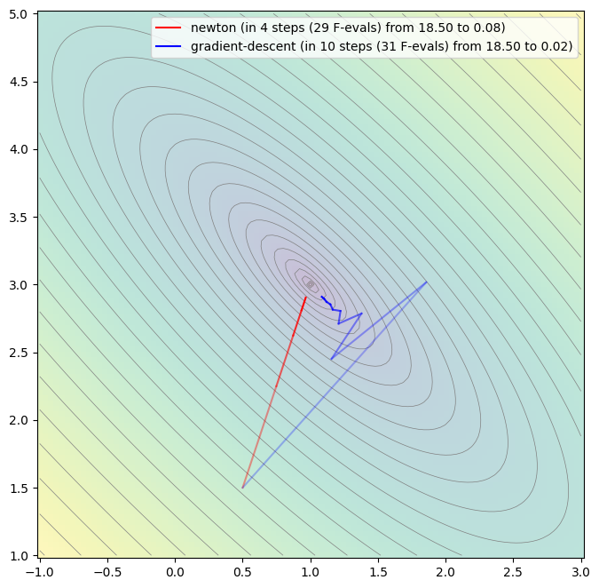
As seen the Newton method finds a much more direct path towards the optimum and requried a fewer number of steps. This can be explained by the mathematical derivation of the Newton method which is designed to converge with quadratic order, whereas basically all other optimization/root-finding methods only converge linearly. On the other hand, each step is associated with much higher numerical costs due to estimation of the Hessian matrix. The meta-parameter in the Newton method is orgiginally set to 1.0 and in case is sufficiently smoot this also leads to the fastest convergence. However, in many cases needs to be used to guarantee convergence which eventually leads to the damped Newton method. For the Booth function, will lead to immidiate convergence after one step. This is due to the fact, that the first derivative of is a linear function and that analytical optimisation is essentially a solution of a linear equation system - precisely the one which is solved in the Newton iteration. The choice of the parameter of the Gradient descent method is much more relevant. If chosen too large, the method will drastically overstep and diverge, if chosen too small, the convergence speed will suffer. For the given setup, eventually leads to divergence, leads to a monotonical convergence. Any value in between will lead to alternating convergence. Easily seen, the steps of the Gradient descent are always orthogonal to the contour lines, whereas the Newton method has a different search direction.
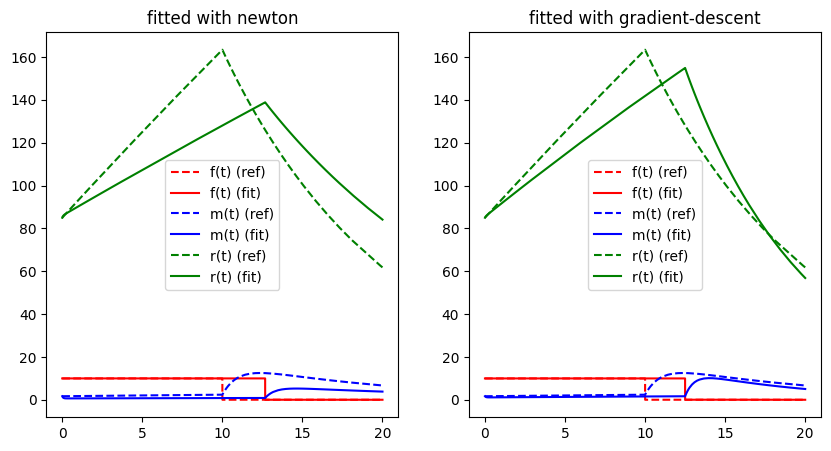
Example: Lithium Cluster Dynamics (Gradient-Based Methods)
As seen, gadient-based methods perform quite well when applied to suitable problems. We wrap the LithiumClusterIndividual and its compute_error and attempt to apply the gradient based methods to fit the first two parameter values (assuming that the other 8 are known). We will wrap the application to help comparing the methods with other algorithms later on.
def visualise_lithium_simulation_fit(
free_parameters: np.ndarray, free_parameter_indices: np.ndarray
) -> None:
"""Visualizes the esults of the Lithium-Cluster model with the fitted and the reference parameters.
:param free_parameters: fitted parameters
:param free_parameter_indices: indices of the free parameters
"""
params = default_params.copy()
model = LithiumClusterModel(params)
T, X = model.run(20) # run the model with the reference parameters
p2arr = embed_free_parameters(free_parameter_indices, free_parameters)
params2 = LithiumClusterConfig()
params2.from_array(p2arr)
model2 = LithiumClusterModel(params2)
T2, X2 = model2.run(20) # run the model with the fitted parameters
plt.plot(T, X[0, :], color="r", linestyle="dashed", label="f(t) (ref)")
plt.plot(T2, X2[0, :], color="r", label="f(t) (fit)")
plt.plot(T, X[1, :], color="b", linestyle="dashed", label="m(t) (ref)")
plt.plot(T2, X2[1, :], color="b", label="m(t) (fit)")
plt.plot(T, X[2, :], color="g", linestyle="dashed", label="r(t) (ref)")
plt.plot(T2, X2[2, :], color="g", label="r(t) (fit)")
lithium_cluster_heatmap_2d = None
def run_lithium_cluster_test(
optimizer: Optimizer | list[Optimizer],
free_parameter_indices: np.ndarray,
max_iters: int | list[int],
):
global lithium_cluster_heatmap_2d
def function(p: np.ndarray): # wrapped lithium cluster model
params = default_params.to_array()
params[free_parameter_indices] = p
config = LithiumClusterConfig()
config.from_array(params)
mdl = LithiumClusterModel(config)
t_sim, x_sim = mdl.run(20)
return error_lithium_cluster(t_sim, x_sim)
if isinstance(optimizer, Optimizer):
optimizer = [optimizer]
if isinstance(max_iters, int):
max_iters = [max_iters for opt in optimizer]
p_sol = extract_free_parameters(
free_parameter_indices, default_params.to_array()
) # (usually unknown) target solution
free_parameter_space = extract_free_parameter_space(free_parameter_indices)
p0 = 0.5 * np.sum(
free_parameter_space, 1
) # pick starting value for iteration right in the middle of the parameter space
plt.figure(figsize=(10, 5))
if (
len(free_parameter_indices) == 2
and free_parameter_indices[0] == 0
and free_parameter_indices[1] == 1
):
## if we solve a 2d problem, plot a heatmap
if lithium_cluster_heatmap_2d is None:
print("compute parameter space heatmap (might take a while)")
lithium_cluster_heatmap_2d = compute_parameter_space_heatmap(
function, 0.5, 2.0, 25, 0.05, 0.15, 25
)
plot_parameter_space_heatmap(*lithium_cluster_heatmap_2d)
plt.scatter(
[p_sol[0]], [p_sol[1]], color="k", marker="x", label="reference minimum"
) # plot the actual global optimum
colors = ["r", "b", "g", "c", "m", "y"]
sols = list()
for i, (opt, m_it) in enumerate(zip(optimizer, max_iters)):
opt.set_function(function)
opt.set_ground_truth(p_sol)
print(
f"##### Start fitting of {len(free_parameter_indices)} dimensional problem with {opt.name.upper()} ####"
)
sol = opt.run(
m_it, p0=p0, color=colors[i % 6]
) # we should not test more than 6 at once anyway ...
sols.append(sol)
plt.legend()
plt.axis("auto")
plt.title(f"fit of {len(free_parameter_indices)} dimensional problem")
plt.figure(figsize=(10, 5))
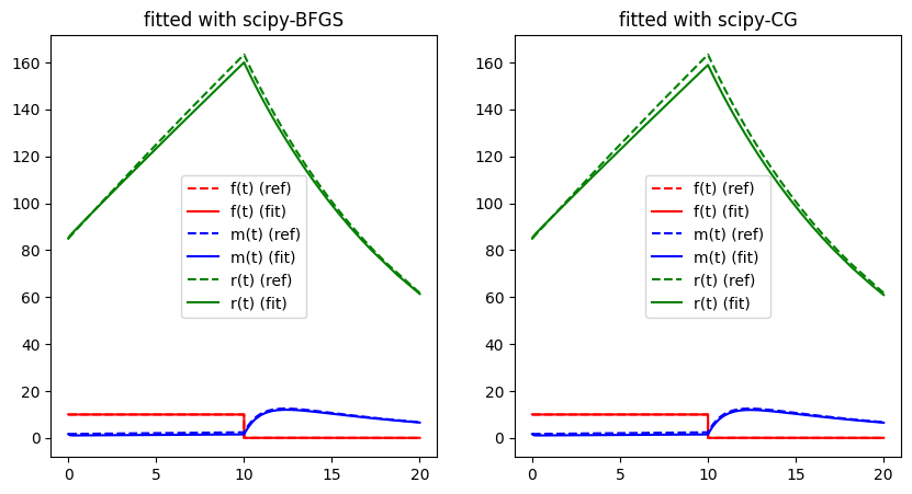
for i, (sol, opt) in enumerate(zip(sols, optimizer)):
plt.subplot(1, len(sols), i + 1)
visualise_lithium_simulation_fit(sol, free_parameter_indices)
plt.legend()
plt.title(f"fitted with {opt.name}")
newton_opt = NewtonOptimizer(None, h=0.001, gamma=0.5)
gradient_opt = GradientDescentOptimizer(None, h=0.001, alpha=0.0000002)
run_lithium_cluster_test([newton_opt, gradient_opt], np.array([0, 1]), [15, 40])
plt.show()compute parameter space heatmap (might take a while)
##### Start fitting of 2 dimensional problem with NEWTON ####
step 0: [1.6   0.125] -> 370.6116275091885
step 1: [1.60355893 0.12021034] -> 274.5011154502478
step 2: [1.60686955 0.10912105] -> 104.68677391223692
step 3: [1.602172 0.11279639] -> 154.58185250673088
step 4: [1.60414196 0.11280215] -> 154.81042913813332
step 5: [1.61628162 0.10630847] -> 76.4063475333004
step 6: [1.61032289 0.09657597] -> 12.726260810928082
step 7: [1.60966591 0.09414851] -> 6.442018345070119
step 8: [1.60753639 0.09276461] -> 4.469274137070675
step 9: [1.58589083 0.09127842] -> 3.7489391415192768
step 10: [1.58564538 0.09114544] -> 3.774755253838519
step 11: [1.58583518 0.09105027] -> 3.7892495828008426
step 12: [1.5853785  0.09096204] -> 3.820375055640502
step 13: [1.5848141  0.09095547] -> 3.839834402753909
step 14: [1.58507339 0.09096577] -> 3.8314763756876675
step 15: [1.58505423 0.09098674] -> 3.8204596738467864
Summary: steps 15, func-evals: 106, accuracy x: 0.5919563676222517, residual: 3.8204596738467864
##### Start fitting of 2 dimensional problem with GRADIENT-DESCENT ####
step 0: [1.6   0.125] -> 370.6116275091885
step 1: [1.59985195 0.12087723] -> 286.5453310681389
step 2: [1.59988238 0.11713013] -> 219.8866721629916
step 3: [1.59981072 0.11377242] -> 167.9362287419802
step 4: [1.59994253 0.11096888] -> 128.97688648951396
step 5: [1.59983185 0.10823137] -> 96.48822313558182
step 6: [1.59979698 0.10597533] -> 73.46656273730048
step 7: [1.59977191 0.10400053] -> 55.93217168966081
step 8: [1.59974891 0.10228241] -> 43.04295613224839
step 9: [1.5997329  0.10082071] -> 33.39225262849807
step 10: [1.59972836 0.09951883] -> 25.926624753349643
step 11: [1.59972158 0.09839719] -> 19.3965978806155
step 12: [1.59970743 0.09721768] -> 14.61157397259421
step 13: [1.59970521 0.09641344] -> 11.857693630222691
step 14: [1.599701   0.09571277] -> 9.736982610375918
step 15: [1.59969696 0.09510314] -> 8.165754377178427
step 16: [1.59968864 0.09456542] -> 6.988103036621226
step 17: [1.59968314 0.09408928] -> 6.1282923788818096
step 18: [1.59968336 0.09367983] -> 5.4511631078026825
step 19: [1.59967509 0.0933215 ] -> 4.996570293194916
step 20: [1.59967466 0.09301103] -> 4.622093936975236
step 21: [1.59967544 0.09274076] -> 4.36364868227001
step 22: [1.59967234 0.09250397] -> 4.194113374359381
step 23: [1.59967473 0.09230072] -> 4.051618075374764
step 24: [1.59967698 0.09211865] -> 3.938384827464199
step 25: [1.59967556 0.09195486] -> 3.8643646757921304
step 26: [1.59967402 0.09181059] -> 3.817414279110336
step 27: [1.59967254 0.09169047] -> 3.791822492756779
step 28: [1.59967438 0.09158319] -> 3.7853810326132713
step 29: [1.5996731  0.09149388] -> 3.748059691664402
step 30: [1.59966753 0.09141252] -> 3.759662201930053
step 31: [1.59967024 0.09133962] -> 3.7692025957888986
step 32: [1.59967314 0.09127757] -> 3.7593568787747245
step 33: [1.59967048 0.09122512] -> 3.751670995653056
step 34: [1.599669   0.09117296] -> 3.7806172856146114
step 35: [1.59966984 0.09113494] -> 3.7804625509887084
step 36: [1.59967401 0.09109781] -> 3.7871268320277403
step 37: [1.59967622 0.0910704 ] -> 3.771815751409889
step 38: [1.59967529 0.09104098] -> 3.7820725930410632
step 39: [1.59967243 0.0910134 ] -> 3.792849491598637
step 40: [1.59967329 0.09099501] -> 3.7911593615053927
Summary: steps 40, func-evals: 121, accuracy x: 0.6063967587287755, residual: 3.7911593615053927
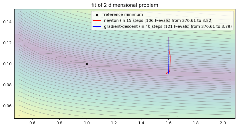

Easily seen, the procedure shows a less clear convergence path due to several local optima of the error function. Clearly, the search space is much more complicated and the numerical computation of the derivatives seems to be numerically problematic. Nevertheless, the procedures seem to converge towards a somewhat satisfactory residual. However, it clearly does not approach the global optimum. Note, that the Gradient descent only appear to be non-orthogonal to the contour lines because axis-scaling is not equal.
It should be noted that Python’s scipy library offers a variety of fully implemented and highly optimised Gradient-based methods such as the mentioned BFGS algorithm (Head & Zerner (1985)) or the Conjugate Gradient (CG) method (Polyak (1969)). We write a quick wrapper-class to include built-in optimizer in our framework.
class SciPyOptimizer(IterativeOptimizer):
    def __init__(
        self, function: Callable[[np.ndarray], float] | None, method_name: str
    ) -> None:
        """Implements the Gradient Descent method
        :param function: function to minimize. Can be None to specify later
        :param h: stepsize for estimation of the gradient
        :param alpha: stepsize for the descent step
        """
        super().__init__(function, name="scipy-" + method_name)
        self.method_name = method_name

    def run(self, max_iter: int, p0: np.ndarray = None, color="r") -> np.ndarray:
        """Runs the scipy optimizer. Max-iter will be ignored.
        :param max_iter: maximum iterations (will be ignored)
        :param p0: initial guess (must be given in this implementation!)
        :param color: color for plotting
        :return: optimized parameter set
        """
        assert p0 is not None, ValueError(
            "Iterative optimizer must have a p0 value which is not None"
        )
        self.reset()
        p = p0.copy()
        fp = self.function_base(p)  # dont count this function evaluation
        self.trajectory.append(p)
        self.fps.append(fp)
        self.print_msg()
        popt = minimize(self.function, x0=p, method=self.method_name)
        p = popt.x
        fp = self.function_base(p)  # dont count this function evaluation
        self.step = popt.nit
        self.trajectory.append(p)
        self.fps.append(fp)
        self.print_msg()
        lbl = f"{self.name} (in {self.step} steps ({self.count} F-evals) from {self.fps[0]:.02f} to {self.fps[-1]:.02f})"
        for i, (x0, x1) in enumerate(zip(self.trajectory[:-1], self.trajectory[1:])):
            plt.plot([x0[0], x1[0]], [x0[1], x1[1]], color=color, alpha=1.0, label=lbl)
        self.print_final_msg()
        return self.trajectory[-1]


bfgs_opt = SciPyOptimizer(None, "BFGS")
cg_opt = SciPyOptimizer(None, "CG")
run_lithium_cluster_test([bfgs_opt, cg_opt], np.array([0, 1]), [0, 0])
plt.show()
##### Start fitting of 2 dimensional problem with SCIPY-BFGS ####
step 0: [1.6 0.125] -> 370.6116275091885
step 2: [1.54901922 0.088346  ] -> 7.6230424225609585
Summary: steps 2, func-evals: 131, accuracy x: 0.5612518827163535, residual: 7.6230424225609585
##### Start fitting of 2 dimensional problem with SCIPY-CG ####
step 0: [1.6   0.125] -> 370.6116275091885
step 1: [1.54736496 0.08715664] -> 10.779056477528993
Summary: steps 1, func-evals: 107, accuracy x: 0.5622309132604023, residual: 10.779056477528993
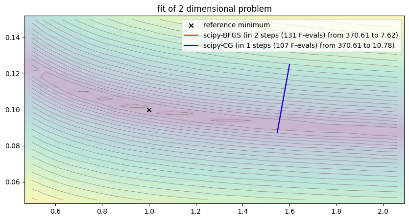
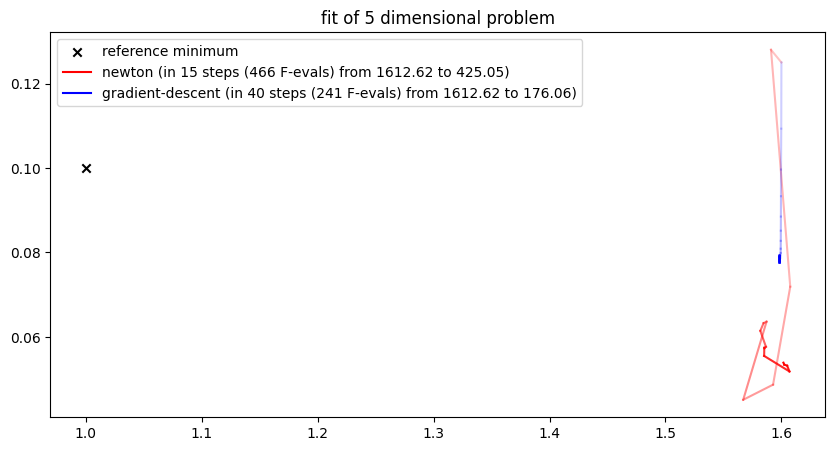
While the methods seem to work somewhat properly for the case study when applied to the two-dimensional problem with free parameters and , we quickly run into troubles when applied to a higher dimensional problem, when trying to fit and at the same time.
newton_opt = NewtonOptimizer(None, h=0.001, gamma=0.5)
gradient_opt = GradientDescentOptimizer(None, h=0.001, alpha=0.0000003)
run_lithium_cluster_test(
    [newton_opt, gradient_opt], np.array([0, 1, 2, 3, 6]), [15, 40]
)
plt.show()
##### Start fitting of 5 dimensional problem with NEWTON ####
step 0: [ 1.6 0.125 0.105 1.65 12.5 ] -> 1612.6191361568735
step 1: [ 1.59102985 0.1279978 0.09991122 1.61654535 12.50157289] -> 1926.068376488872
step 2: [ 1.60761839 0.07190269 0.093779 1.55583198 12.61298065] -> 331.55556025496264
step 3: [ 1.59280716 0.04870346 0.014707 1.62362804 12.61401261] -> 1009.4315644541135
step 4: [ 1.56705886 0.04512411 0.0333314 1.6150517 12.63223689] -> 693.0801886143115
step 5: [ 1.58716878 0.06361735 0.08131261 1.59779625 12.63366993] -> 364.58840847769244
step 6: [ 1.5845945 0.06326995 0.08457507 1.59851742 12.634279 ] -> 344.5978254752904
step 7: [ 1.58181498 0.06145599 0.08743642 1.59762789 12.6376272 ] -> 330.2454414527948
step 8: [ 1.58665591 0.05766413 0.08257363 1.61100579 12.6358751 ] -> 356.5597866482519
step 9: [ 1.58532562 0.05733326 0.08392225 1.61110282 12.63446836] -> 351.5084512084837
step 10: [ 1.58523292 0.05743923 0.08255205 1.61114571 12.63400155] -> 355.8174183416166
step 11: [ 1.58511799 0.05550659 0.08405395 1.61086593 12.6346334 ] -> 360.46872213377685
step 12: [ 1.60693016 0.0518322 0.07159212 1.58591492 12.63265495] -> 419.7763244519312
step 13: [ 1.6049331 0.05320062 0.0709221 1.58706864 12.63426053] -> 415.77740632998547
step 14: [ 1.60244709 0.05344962 0.07272252 1.58012534 12.64369796] -> 408.47553377560934
step 15: [ 1.60174707  0.05390892  0.06984138  1.57404939 12.67223531] -> 425.0542219891589
Summary: steps 15, func-evals: 466, accuracy x: 1.0326827273133912, residual: 425.0542219891589
##### Start fitting of 5 dimensional problem with GRADIENT-DESCENT ####
step 0: [ 1.6    0.125  0.105  1.65  12.5  ] -> 1612.6191361568735
step 1: [ 1.59986876  0.10931882  0.11381232  1.65020944 12.4998393 ] -> 803.781072548793
step 2: [ 1.599655    0.09964003  0.11835735  1.65034162 12.49964935] -> 489.594521346261
step 3: [ 1.59961841  0.09331891  0.12164544  1.65050509 12.4995028 ] -> 343.3262250757165
step 4: [ 1.59954506  0.08850256  0.12376906  1.65056058 12.49940285] -> 266.65455779268706
step 5: [ 1.59949094  0.08516115  0.12541532  1.65060826 12.49932228] -> 228.2856792116889
step 6: [ 1.59944613  0.08276024  0.12657584  1.65064376 12.49926639] -> 207.93465275235465
step 7: [ 1.59937084  0.08089328  0.12744054  1.65072324 12.49923156] -> 198.09689183451158
step 8: [ 1.59935258  0.07986218  0.12845403  1.65068869 12.49917692] -> 192.1050430218511
step 9: [ 1.59893629  0.07911829  0.12915991  1.65072308 12.49914486] -> 189.14927784651766
step 10: [ 1.59883841  0.07859196  0.12957275  1.65087688 12.49910166] -> 187.8700564803508
step 11: [ 1.59840353  0.07814287  0.13020781  1.65092435 12.49905892] -> 186.24914870129788
step 12: [ 1.59847105  0.07795897  0.13076535  1.65095951 12.49901077] -> 184.89639781774494
step 13: [ 1.59840197  0.07768927  0.13115847  1.650939   12.49896892] -> 184.46324752892576
step 14: [ 1.59841919  0.07757629  0.13154609  1.65095558 12.49895613] -> 183.92426268210323
step 15: [ 1.5984191   0.0775543   0.1318705   1.65095535 12.49891585] -> 183.55616058439378
step 16: [ 1.59842769  0.07753288  0.13219388  1.65095374 12.49887393] -> 183.21167130175027
step 17: [ 1.59843336  0.07759756  0.13250766  1.65095486 12.49882559] -> 182.85624811487446
step 18: [ 1.59844311  0.07767632  0.13282509  1.65096237 12.49878756] -> 182.42401682418745
step 19: [ 1.59844496  0.07775062  0.13312339  1.65095917 12.49873854] -> 182.06655349649816
step 20: [ 1.59844637  0.07782275  0.13342013  1.65095885 12.4987021 ] -> 181.71336471591363
step 21: [ 1.59844578 0.07790179 0.13371218 1.65095821 12.49866659] -> 181.35731702076603
step 22: [ 1.59844804 0.07797422 0.13399918 1.65095647 12.49862909] -> 180.99844218667107
step 23: [ 1.59843967 0.07804386 0.13427044 1.65094431 12.4985849 ] -> 180.7244246259211
step 24: [ 1.59844364  0.07812944  0.13455148  1.65094463 12.49854739] -> 180.38067802583848
step 25: [ 1.59844208  0.07820868  0.13482628  1.65094563 12.4985131 ] -> 180.053305795491
step 26: [ 1.59845123  0.07828068  0.13509627  1.65094289 12.49847253] -> 179.74796357325744
step 27: [ 1.59845259  0.0783657   0.13536222  1.65093961 12.4984325 ] -> 179.45196632046157
step 28: [ 1.59845383  0.0784508   0.135631    1.65093764 12.49839519] -> 179.112801129654
step 29: [ 1.59844909  0.07851309  0.13588346  1.650929   12.49835123] -> 178.86707958454335
step 30: [ 1.59845486  0.07858931  0.13614067  1.65092906 12.49831448] -> 178.58440020907085
step 31: [ 1.59845501  0.07866485  0.13639868  1.65093759 12.49827913] -> 178.30300237046507
step 32: [ 1.59845421  0.07873693  0.13665582  1.65093576 12.49824592] -> 178.02241251325873
step 33: [ 1.59845917  0.07881465  0.13690538  1.65094356 12.49820997] -> 177.75926119882894
step 34: [ 1.59846481  0.07888839  0.13715656  1.65094638 12.49817849] -> 177.4809280027195
step 35: [ 1.59847014  0.07896501  0.13739423  1.6509437  12.49813857] -> 177.22464459954463
step 36: [ 1.59847003 0.07903279 0.13763199 1.65094305 12.49810314] -> 176.97454549899442
step 37: [ 1.59847319 0.07910296 0.13786272 1.65094395 12.49806632] -> 176.74062141981526
step 38: [ 1.59847532 0.07917943 0.13809429 1.65094396 12.49803044] -> 176.48842054824001
step 39: [ 1.59847298  0.07924942  0.1383189   1.65093759 12.49799661] -> 176.26113965909255
step 40: [ 1.59846721  0.0793192   0.13853492  1.65093357 12.49796598] -> 176.06230946047066
Summary: steps 40, func-evals: 241, accuracy x: 1.0176145814972342, residual: 176.06230946047066
Metaheuristics
Methods such as the Newton’s method approaches are derived purely mathematically and provide guaranteed convergence towards an optimum, however only under certain prerequisites, such as two-times differentiability of the objective function, i.e. that mut be twice differentiable w.r. to . Moreover, they are designed to converge towards the closest local optimum which may differ from the global one. Finally, it is almost impossible to add additional constraints to the parameter vector, e.g. to ensure that it remains within the parameter space or to make sure that it only takes integer values.
To overcome these constraints, heuristics and metaheuristics can be applied. The latter is an umbrella term for a large collection of search algorithms, which can be applied to find a global optimum. These algorithms are designed to converge towards an optimum, however not derived from mathematics but inspired by natural processes and/or causal logic. As described in Blum & Roli (2003) metaheuristics are often stochastic and their field or application can vary. While some methods are very problem specific, e.g. ant colony optimisation was developed specifically for optimising path lengths on graphs, some others are very universal, e.g. a genetic algorithm can in priciple be applied to any optimisation problem. Since metaheuristics, unlike gradient-based methods, generally do not offer any formal convergence guarantees, they can and must usually be tuned using a larger number of hyperparameters or, in some cases, even hyper-processes. The success of their application depends on choosing these appropriately.
Conventionally, in the terminology of metaheusristics, the parametervector is usually referred to as individual and the error is associated with the fitness of the individual, e.g. a fitness-value could be defined by or . A metaheuristic is usually formalised to find the individual with the highest fitness, which, of course, is identical to the orginal problem of finding a parameterset with the smallest error.
Local vs Global Search Algorithms
The field of metaheuristics can be classified in many different ways. The most important classification is that into local and global search algorithms. The former, like gradient-based methods, attempt to converge to the nearest local optimum, whilst the latter always aim to find the global optimum. The most simplistic local search strategy is the hill-climbing or mountain-climbing algorithm.
Hill-Climbing Algorithm
Analogous to gradient based methods, the hill-climbing algorithm, to be precise, the stochastic hill climbing algorithm iteratively improves a given initial estimate w.r. to a given objetive function . However, instead of approxmation of a gradient for finding the next iteration step, the method uses stochasticiy. In order to find the next step, the algorithm slightly alters the current individual of the algorithm by a random noise to get an altered individual . Thereafter, it compares the fitness of the original and the altered individual. If yields a smaller error as the one before, is accepted as the new state of the algoritm, if not, the algoritm continues with . We may formalise this as
Hereby, is a realisation of a stochastic variable with and is a stepwidth. The optional mapping maps the modified individual onto the parameter-space . The algorithm offers lots of freedom for customisation with respect to hyperparameters/hyperprocesses. E.g.
the distribution for could be discrete or hybrid to make sure that certain parameters remain integer valued,
the step-width could depend on the size of the parameterspace and/or on the iteration count.
| Hyperparameter | Symbol | Range/Space | Considerations |
|---|---|---|---|
| distribution for stochastic modification of the parameterset | continuous/discrete/hybrid distribution with | When the parameterspace is discrete (i.e. a lattice) choose to randomly draw from a grid-neighbour, if it is continuous a mulidimensional normal distribution often works nicely. | |
| stepwidth for stochastic modification of the parameterset | positive scalar | can be constant, however it is advised to have it decrease with the iteration count, e.g. by for some small positive . | |
| Parameter space mapping | with | Could be if the parameter space is unbounded or no bounds are known. Otherwise, it should map any potential modified individual outside the parameter-space back into the parameterspace. |
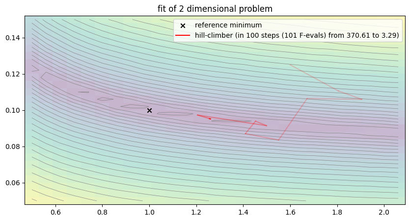
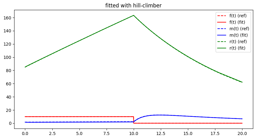
Example: Lithium Cluster Dynamics (Hill-Climbing Algorithm)
The hill-climbing algorithm applies straight forwardly to the case study. We use the function
whereas and are the lower and upper boundaries of the parameter-space for every coordinate, to make sure that the algorithm does not leave the parameterspace.
class HillClimbingOptimizer(IterativeOptimizer):
    def __init__(
        self,
        function: Callable[[np.ndarray], float] | None,
        parameter_space: np.ndarray,
        alpha=0.1,
    ) -> None:
        """Optimizer using a stochastic Hill Climbing algorithm
        :param function: function to minimize. Can be None to specify later
        :param parameter_space: boundaries of the parameter space
        :param alpha: "stepwidth", i.e. relative standarddeviation of the normal distribution.
        """
        super().__init__(function, name="hill-climber")
        self.parameter_space_lb = parameter_space[:, 0]
        self.parameter_space_up = parameter_space[:, 1]
        self.parameter_diff = self.parameter_space_up - self.parameter_space_lb
        self.alpha = alpha

    def map_to_parameterspace(self, p: np.ndarray) -> np.ndarray:
        """Maps a parameter vector (back) onto the parameterspace
        :param p: parameter vector
        :return: parameter vector mapped onto the parameterspace
        """
        return np.minimum(
            self.parameter_space_up, np.maximum(self.parameter_space_lb, p)
        )

    def mutate(self, p: np.ndarray) -> np.ndarray:
        """Performs a stochastic mutation of a parameter vector
        :param p: parameter vector
        :return: new mutated parameter vector
        """
        dim = len(p)
        X = np.random.randn(dim)
        alpha = self.alpha * 0.99**self.step
        return p + X * self.parameter_diff * alpha

    def update_step(self, p: np.ndarray, fp: float) -> tuple[np.ndarray, float | None]:
        """Performs a stocahstic hill climber step.
        Randomly mutates the parameter vector, maps it back onto the parameter space and accepts the mutation if it produces a lower error as the original.
        :param p: current status of the iteration
        :param fp: function value at p
        :return: updated state
        """
        p2 = self.mutate(p)
        p2 = self.map_to_parameterspace(p2)
        fp2 = self.function(p2)
        if fp2 < fp:
            return p2, fp2
        return p, fp


np.random.seed(12346)  # fix random seed (has quites om influence, try to vary it!)
free_parameter_indices = np.array([0, 1])
hc_opt = HillClimbingOptimizer(
    None,
    alpha=0.1,
    parameter_space=extract_free_parameter_space(free_parameter_indices),
)
run_lithium_cluster_test(hc_opt, free_parameter_indices, 100)
free_parameter_indices = np.array([0, 1, 2, 3, 6])
hc_opt = HillClimbingOptimizer(
    None,
    alpha=0.1,
    parameter_space=extract_free_parameter_space(free_parameter_indices),
)
run_lithium_cluster_test(hc_opt, free_parameter_indices, 200)
plt.show()
##### Start fitting of 2 dimensional problem with HILL-CLIMBER ####
step 0: [1.6 0.125] -> 370.6116275091885
step 2: [1.80536438 0.11057051] -> 148.35996504379165
step 3: [1.90473964 0.1059794 ] -> 101.59026623294581
step 4: [1.67177785 0.10638079] -> 85.96653703495558
step 5: [1.55046255 0.08353004] -> 24.264827979838326
step 8: [1.40927466 0.08704452] -> 15.343470501162829
step 13: [1.45237225 0.09392101] -> 3.9328056781398066
step 16: [1.49918734 0.09144489] -> 3.776879098222401
step 20: [1.20525659 0.0973088 ] -> 3.544423770564969
step 25: [1.26048866 0.09517081] -> 3.290522923262052
step 91: [1.25599064 0.09530826] -> 3.285058245138312
Summary: steps 100, func-evals: 101, accuracy x: 0.2602545812683573, residual: 3.285058245138312
##### Start fitting of 5 dimensional problem with HILL-CLIMBER ####
step 0: [ 1.6    0.125  0.105  1.65  12.5  ] -> 1612.6191361568735
step 1: [ 1.46214371  0.13056893  0.13797148  1.6409395  11.04698434] -> 285.975302945007
step 2: [0.84040805 0.13009243 0.12899171 1.53982612 9.69922651] -> 118.81172614969631
step 8: [ 0.95167883 0.12520384 0.12618013 1.67199473 10.57289737] -> 33.10398818878504
step 16: [ 1.06135493 0.11951868 0.11768697 1.80495956 10.16627723] -> 26.294371872161268
step 36: [1.31994776 0.10759117 0.10564893 1.90922304 9.96354763] -> 22.526640396656255
step 53: [1.19233889 0.11367147 0.09238479 1.93317246 9.77542888] -> 19.246849144114297
step 83: [ 1.18542841 0.11498316 0.10948219 1.83485011 10.14918948] -> 14.862444744244712
step 135: [ 1.05973022  0.11262397  0.10134884  1.77016565 10.00059505] -> 13.55666218400145
step 140: [1.06082012 0.11409082 0.10342073 1.71726677 9.97651913] -> 12.251937925149484
step 147: [ 1.06374959 0.11227189 0.10183897 1.72470998 10.03078454] -> 11.856172518733763
step 175: [ 1.05615655  0.11199042  0.09833978  1.71971588 10.03990562] -> 11.524475036597979
step 181: [ 1.02584499  0.11018978  0.10218445  1.66962361 10.17679059] -> 11.059882059938035
step 197: [ 1.01267885  0.11072853  0.10390619  1.63942593 10.18669905] -> 10.564190183343221
Summary: steps 200, func-evals: 201, accuracy x: 0.649931389004793, residual: 10.564190183343221
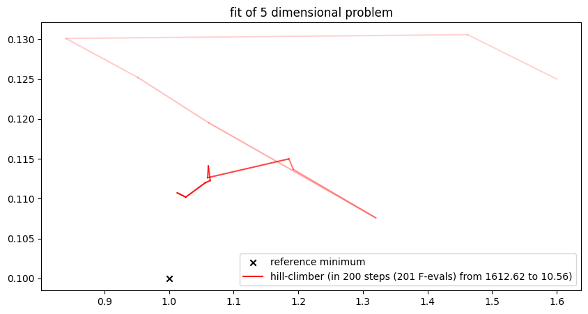
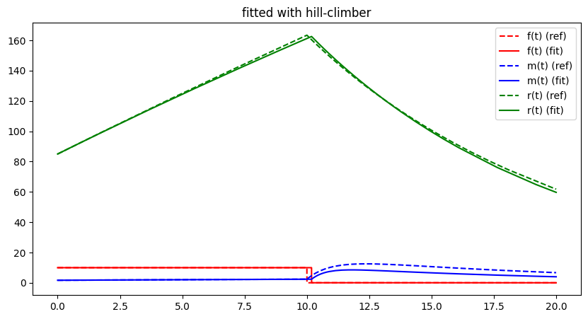
Although the algorithm seems to work properly not only for the 2-d problem but also for the 5-d problem, by design, convergence towards the global optimum is essentially a coin-flip. In most cases, a local but not global optimum will be approached. Global search strategies aim to avoid this by adding additional ideas to leave local optimal / local valleys. The most straight forward of these methods directly extends the Hill Climbing algorithm:
Simulated Annealing
Simulated Annealing essentially uses the same update step as the Hill Climbing algorithm, with the sole difference being that a parameterset modified to the “worse”, i.e , is not automatically discarded, but is accepted with a certain probability, see Bertsimas & Tsitsiklis (1993). The algorithm can be formalised as
Analogous to the Hill Climbing algorithm, is a realisation of a stochastic variable with and is a stepwidth. Moreover, refers to a uniformly distributed number and the exponential term is the acceptance probability. The most crucial parameter, however, is the scaling term which is usually referred to as temperature. The higher, the temperature, the higher the probability for accepting a step into the “wrong direction”.
The key idea of Simulated Annealing is to start with a comparably large temperature and lower it iteratively with every step, i.e. . Hereby, the algorithm may initially explore the parameterspace without committing to a local optimum too soon. After a while, becomes very small and the method essentially becomes a Hill Climbing strategy to converge properly. This idea is inspired by the qualitative behaviour of metal while forging. The material remains flexible for deformation while hot and becomes more and more sturdy when cooling down.
This adds one new hyperparameter to the ones from the Hill Climbing algorithm:
| Hyperparameter | Symbol | Range/Space | Considerations |
|---|---|---|---|
| sequence of temperaure values | positive real numbers with | declining sequence, e.g. for some small . The starting value must reflect the size of error at the start of the iteration. | |
| distribution for stochastic modification of the parameterset | continuous/discrete/hybrid distribution with | When the parameterspace is discrete (i.e. a lattice) choose to randomly draw from a grid-neighbour, if it is continuous a mulidimensional normal distribution often works nicely. | |
| stepwidth for stochastic modification of the parameterset | positive scalar | can be constant, however it is advised to have it decrease with the iteration count, e.g. by for some small positive . | |
| Parameter space mapping | with $\forall x\in P: | ||
| g(x)=x$ | Could be if the parameter space is unbounded or no bounds are known. Otherwise, it should map any potential modified individual outside the parameter-space back into the parameterspace. |
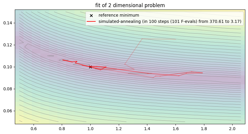
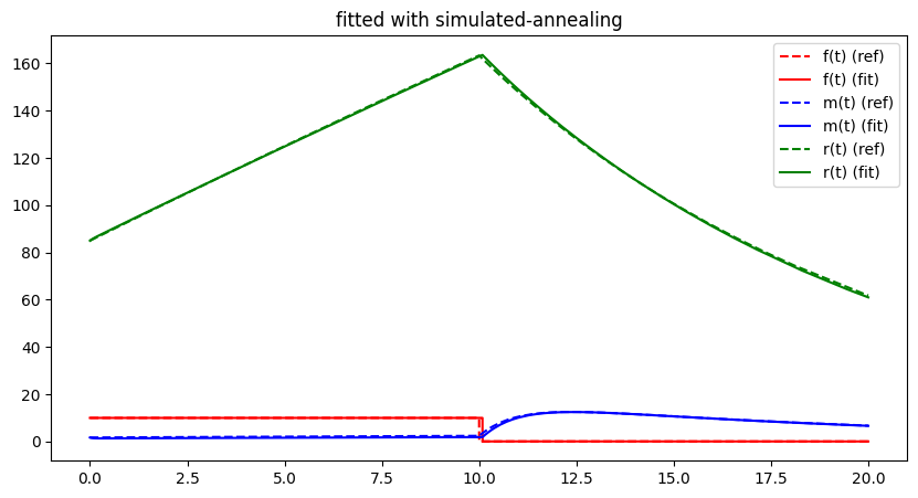
Case Study: Lithium Cluster Dynamics - Simulated Annealing
Below we implemented a variant of the Simulated Annealing algorithm specifcally designed for the lithium-cluster case-study. Since the search space does contain several of local optima, the temperature parameter should not decline too fast.
class SimulatedAnnealingOptimizer(HillClimbingOptimizer):
    def __init__(
        self,
        function: Callable[[np.ndarray], float] | None,
        parameter_space: np.ndarray,
        alpha: float = 0.1,
        t0: float = 10.0,
        qt: float = 0.95,
    ) -> None:
        """Optimizer using a Simulated Annealing
        :param function: function to minimize. Can be None to specify later
        :param parameter_space: boundaries of the parameter space
        :param alpha: "stepwidth" for mutation, i.e. relative standarddeviation of the normal distribution.
        :param t0: initial temperature
        :param qt: decline of temperature per step
        """
        super().__init__(function, parameter_space, alpha)
        self.name = "simulated-annealing"
        self.t0 = t0
        self.qt = qt

    def update_step(self, p: np.ndarray, fp: float) -> tuple[np.ndarray, float | None]:
        """:param p: current status of the iteration
        :param fp: function value at p
        :return: updated state
        """
        p2 = self.mutate(p)
        p2 = self.map_to_parameterspace(p2)
        fp2 = self.function(p2)
        if fp2 < fp:
            return p2, fp2
        t = self.t0 * self.qt**self.step
        if np.random.random() < np.exp(-(fp2 - fp) / t):
            return p2, fp2
        return p, fp


np.random.seed(12346)
free_parameter_indices = np.array([0, 1])
hc_opt = SimulatedAnnealingOptimizer(
    None,
    alpha=0.1,
    parameter_space=extract_free_parameter_space(free_parameter_indices),
    t0=10,
    qt=0.95,
)
run_lithium_cluster_test(hc_opt, free_parameter_indices, 100)
free_parameter_indices = np.array([0, 1, 2, 3, 6])
hc_opt = SimulatedAnnealingOptimizer(
    None,
    alpha=0.1,
    parameter_space=extract_free_parameter_space(free_parameter_indices),
    t0=10,
    qt=0.95,
)
run_lithium_cluster_test(hc_opt, free_parameter_indices, 200)
plt.show()
##### Start fitting of 2 dimensional problem with SIMULATED-ANNEALING ####
step 0: [1.6 0.125] -> 370.6116275091885
step 3: [1.36468506 0.12540544] -> 306.3135505004997
step 4: [1.24214436 0.10232387] -> 16.490240546194883
step 5: [1.3082493 0.0977372] -> 6.224684626857945
step 6: [1.08451162 0.0977437 ] -> 3.2328914341915347
step 7: [0.94189759 0.10129369] -> 3.165429539956776
step 8: [1.4423167 0.0902276] -> 5.7127317402603515
step 11: [1.45964446 0.09153008] -> 3.973450832937535
step 19: [1.49099077 0.09152134] -> 3.779744552003779
step 25: [1.71350019 0.09548892] -> 12.588822270653123
step 28: [1.78873266 0.09445275] -> 11.490008398507628
step 29: [1.67681378 0.09404913] -> 7.654809381470765
step 30: [1.62314712 0.09183614] -> 3.9734338301702787
step 37: [1.40579742 0.09405884] -> 3.612289274946221
step 41: [1.04630887 0.10030125] -> 3.379452144756268
step 42: [0.99256149 0.10042964] -> 3.0526229044355073
step 45: [1.11123311 0.09989562] -> 4.321218013988341
step 52: [1.07200999 0.09724352] -> 3.8687769734342696
step 66: [0.89417333 0.10353523] -> 3.0921098229766324
step 67: [0.90602963 0.10484258] -> 4.156727672596412
step 68: [0.90036185 0.10501578] -> 4.15832872141182
step 73: [0.8721127  0.10441172] -> 3.2114644399656695
step 94: [0.80633585 0.10620432] -> 3.174113536069359
Summary: steps 100, func-evals: 101, accuracy x: 0.20335968044624825, residual: 3.174113536069359
##### Start fitting of 5 dimensional problem with SIMULATED-ANNEALING ####
step 0: [ 1.6    0.125  0.105  1.65  12.5  ] -> 1612.6191361568735
step 1: [ 1.75349255  0.10131536  0.13302116  1.70229548 13.54529631] -> 978.6376301660877
step 2: [ 2.12198439  0.09562953  0.12622272  1.5194947  12.19617473] -> 381.0800468236381
step 5: [ 1.82034655  0.09020506  0.09627266  1.75309702 11.92580544] -> 335.42578591807256
step 7: [ 1.3812937   0.09011119  0.10017705  1.4716705  10.35979136] -> 23.56438649995806
step 10: [ 1.35305486  0.09782029  0.10384215  1.63907515 10.24045698] -> 17.214635371974826
step 28: [1.26296778 0.10772164 0.11164928 1.49214845 9.96183735] -> 17.54484142927536
step 35: [1.11005374 0.11500768 0.09575483 1.5208471 9.73641417] -> 19.208880353115998
step 78: [ 1.09153358 0.10261095 0.09561584 1.63683908 10.09736914] -> 17.232005678639077
step 92: [1.15965849 0.10624203 0.09935385 1.50239568 9.77879099] -> 15.026976834332238
step 95: [ 0.98043646  0.10522344  0.10168443  1.46376992 10.41259504] -> 14.806663298423029
step 115: [ 1.13767314  0.10011613  0.10363196  1.30885549 10.18862286] -> 6.727434622073158
step 118: [ 1.27878779  0.10196531  0.10586432  1.13382725 10.03138082] -> 6.327897495128162
step 136: [ 1.36216405 0.0991005 0.10268989 1.19438666 10.11380833] -> 6.286043756182625
step 152: [1.29050604 0.09961294 0.10067303 1.09559597 9.84880571] -> 4.578177187274235
step 156: [ 1.3345287   0.09407987  0.10090893  1.06567611 10.07144163] -> 3.657536940497204
step 163: [ 1.31599928 0.09483808 0.10333204 1.02317728 10.08538634] -> 3.2221506793002925
Summary: steps 200, func-evals: 201, accuracy x: 0.3228628634333318, residual: 3.2221506793002925
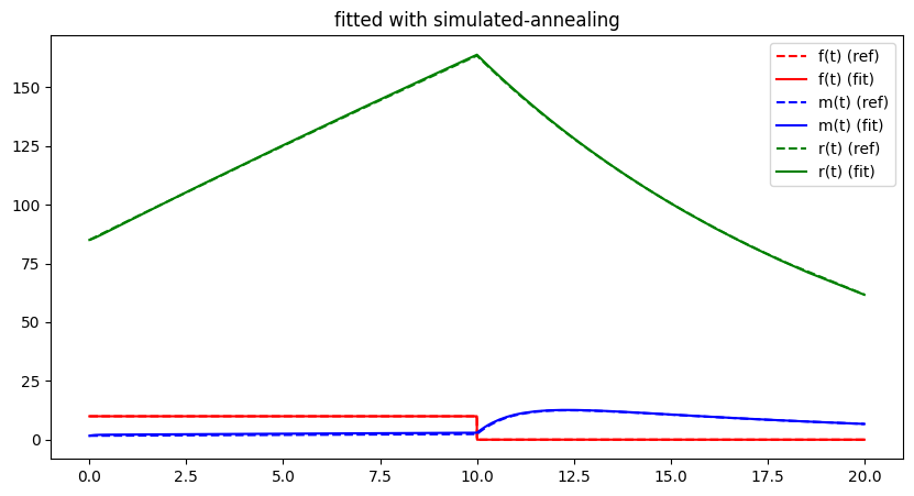
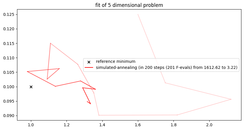
Although simulated annealing increases the likelihood of converging to a global optimum, there is still a significant element of chance involved. The idea of updating an entire population rather than a single individual is intended to counteract this.
Trajectory vs. Population-Based Metaheuristics
Algorithms like Hill Climing and Simulated Annealing are classified as trajectory-based metaheuristics. This name originates from the idea that a single individual is modified and its iteration orbit describes a trajetory in the -dimensional space ( being the number of free parameters). This class of algorithms can be distinguished from the second large class of metaheristics, the population-based. Here, algorithms simultaneously update a whole population of individuals at the same time, which enables a broader search space. That means, instead of updating a single individidual , we update a whole population
Genetic-Algorithm
The most famous class of population-based metaheuristics are genetic algorithms sometimes refered to genetic programming or evolutionary algorithms. The idea of this algorithm is inspired by evolutionary dynamics observed in nature as discovered by Charles Darvin. The iterative algorithm initializes a starting population of individuals and updated this population simultaneously in an iteration. In every update step the three evolutionary mechanisms crossover, mutation and selection are applied as seen in the picure below.
In the crossover process, a number of pairs of individuals are selected for generation of offspring. For each pair of parents an offspring is usually created by randomly selecting if a parameter value is inherited by the one or the other parent, i.e. for two individuals the crossover would be computed by
with distributed random numbers .
In the mutation process, a number of individals are selected to create new individuals via modification. This is usually implemented analogous to the update process in the Simulated Annealing or the Hill Climbing algorithm, however, the origin individual is not discarded. In some implementations, mutation is decided per free parameter, i.e. not every parameter is mutated, i.e.
for some mutation probabilty and an element-wise mutation function .
Finally, the selection process is applied. For this, the individuals are ranked by fitness and the least fit individuals are discarded. In most cases, the number of discarded individuals is matched to the sum of new individuals generated in the course of the mutation and crossover processes.
In general Genetic Algorithms come with a huge degree of freedom w.r. to hyperparameters which can be interpreted as a pro and con at the same time. On the one hand the algorithm can be well tuned to enable good convergence properties, on the other hand a lot of hyperparameter search needs to be performed by the user. We only give a rough idea of the hyperparameters and hyperprocesses:
| Hyperparameter | Symbol | Range/Space | Considerations |
|---|---|---|---|
| size of the population | integer greater than 1 | Reasonable sizes depend on the dimension of the problem. In most cases values between 20 and 200 are used. | |
| distribution of initial individuals | - | some mapping | In most implementations, the initial individuals is drawn uniformly from the parameter space. However, also a more homogeneous mapping is possible using deterministic space-filling sequencese, such as the Sobol sequence Sobol (1967). |
| number and criteria for choosing individuals for mutation and crossover | - | - | Usually the selection probability is influenced by the fitness, i.e. fitter individuals are given higher probaility for being selected to produce offspring or mutants. There is no limitation to the number of new created offsprings or mutants. |
| mutation process | - | - | Mutation process should also consider limitations of the parameter space. Note that the parameter space cannot be left via crossover, which is a big benefit. |
| criteria for choosing individuals for the selection process | - | - | While it makes sense to simply discard the weakest performing part of the population list when sorted by their fitness, nowadays approaches also make sure that genetic diversity is maintained. I.e. that the remainig part of the list is sufficiently different w.r. to some metric on . |
| supporting processes | - | - | In general the algorithm can be extended by additional processes like random resamping or by splitting into two competing subpopulations. Whateher helps the algorithm to converge is viable. |

Example: Lithium Cluster Dynamics (Genetic-Algorithm)
We use a completely straight forward implementation for the lithium-cluster case study.
class PopulationBasedOptimizer(Optimizer):
    def __init__(
        self,
        function: Callable[[np.ndarray], float] | None,
        name: str,
        parameter_space: np.ndarray,
    ) -> None:
        """Base class for a population-based optimization metaheuristic.
        :param function: function to minimize, can be None and speficied later
        :param name: name of the method
        :param parameter_space: for all population-based methods we consider parameter bounds
        """
        super().__init__(function, name)
        self.segments: dict[int, list[tuple[np.ndarray, np.ndarray]]] = (
            dict()
        )  # for plotting
        self.population: list[np.ndarray] = list()
        self.fvals: list[float] = list()
        self.min_fvals: list[float] = list()
        self.step = 0
        self.parameter_space = parameter_space
        self.parameter_space_lb = parameter_space[:, 0]
        self.parameter_space_up = parameter_space[:, 1]
        self.parameter_diff = self.parameter_space_up - self.parameter_space_lb

    def map_to_parameterspace(self, p: np.ndarray) -> np.ndarray:
        """Default method to map a parameter vector back into the parameter space
        :param p: parameter vector draft
        :return: parameter vector mapped into bounds
        """
        return np.minimum(
            self.parameter_space_up, np.maximum(self.parameter_space_lb, p)
        )

    def reset(self) -> None:
        """Resets the counter
        :return:
        """
        super().reset()
        self.segments = dict()
        self.population = list()
        self.fvals = list()
        self.min_fvals = list()
        self.step = 0

    @abstractmethod
    def create_population(self) -> tuple[list[np.ndarray], list[float | None]]:
        """Abstract method to initialize the population
        :return: list of parameter vectors and corresponding list of function values (can be None)
        """
        return list(), list()

    @abstractmethod
    def update_population(
        self, pop: list[np.ndarray], fpop: list[float]
    ) -> tuple[list[np.ndarray], list[float | None]]:
        """Abstract method to performs an update step for the population
        :param pop: current population, i.e. list of parameter vectors
        :param fpop: corresponding list of function values
        :return: updated list of parameter vectors and corresponding list of function values (can be None)
        """
        return list(), list()

    def print_msg(self) -> None:
        """Prints a message to analyze the convergence status at the current step
        :return:
        """
        mn = self.min_fvals[-1]
        i = self.fvals.index(mn)
        print(
            f"step {self.step}: best individual is {self.population[i]} with min error {mn}, max error {max(self.fvals)}"
        )

    def print_final_msg(self) -> None:
        """Prints a summary message after the iteration
        :return:
        """
        mn = self.min_fvals[-1]
        i = self.fvals.index(mn)
        opt = self.population[i]
        if self.p_sol is not None:
            diff = opt - self.p_sol
            reldiff = diff / self.p_sol
            accx = np.linalg.norm(reldiff)
        else:
            accx = "undef."
        print(
            f"Summary: steps {self.step}, func-evals: {self.count}, accuracy x: {accx}, residual: {self.function_base(opt)}"
        )

    def compute_missing_fvals(
        self, pop: list[np.ndarray], fpop: list[float | None]
    ) -> list[float]:
        """Computes all not yet computed function values to the current population
        :param pop: current population, i.e. list of parameter vectors
        :param fpop: corresponding list of function values with potential None entires
        :return: complete list of function values
        """
        fun = lambda x: x[1] if x[1] is not None else self.function(x[0])
        fpop2 = list(map(fun, zip(pop, fpop)))  # this could be parallelised nicely!
        return fpop2

    def run(self, max_iter: int, p0: np.ndarray = None, color="r") -> np.ndarray:
        """Runs the iteration until (at most) max_iter (depending on the implementation of "stop").
        :param max_iter: maximum iterations
        :param p0: initial guess (will be ignored here)
        :param color: color for plotting
        :return: optimized parameter set
        """
        self.reset()
        # initialise population
        self.population, errs = self.create_population()
        self.fvals = self.compute_missing_fvals(self.population, errs)
        self.min_fvals = [min(self.fvals)]

        # print initial conditions
        self.print_msg()
        # start iteration
        for i in range(max_iter):
            self.step = i + 1
            self.segments[self.step] = list()
            self.population, fvs = self.update_population(self.population, self.fvals)
            self.fvals = self.compute_missing_fvals(self.population, fvs)
            self.min_fvals.append(min(self.fvals))
            self.print_msg()
            if self.stop():
                break
        mn = min(self.fvals)
        imn = self.fvals.index(mn)
        pmn = self.population[imn]

        lbl = f"{self.name} (in {i + 1} steps ({self.count} F-evals) from {self.min_fvals[0]:.02f} to {self.min_fvals[-1]:.02f})"
        n = max(self.segments.keys())
        for i, segs in self.segments.items():
            xs = list()
            ys = list()
            for s1, s2 in segs:
                xs.extend([s1[0], s2[0], None])
                ys.extend([s1[1], s2[1], None])
            plt.plot(
                xs,
                ys,
                color=color,
                alpha=i / n,
                linewidth=i / n,
                label=lbl if i == n else None,
            )
        self.print_final_msg()
        return pmn


class GeneticAlgorithmOptimizer(PopulationBasedOptimizer):
    def __init__(
        self,
        function: Callable[[np.ndarray], float] | None,
        parameter_space: np.ndarray,
        pop_size: int = 50,
        crossover_size: int = 10,
        mutate_size: int = 10,
        pm: float = 0.5,
        alpha: float = 0.01,
    ) -> None:
        """Optimizer using a simple genetic algorithm
        :param function: callable function to minimize. Can be None and specified later
        :param parameter_space: boudaries of the parameter space
        :param pop_size: size of the population
        :param crossover_size: number of individuals to crossover
        :param mutate_size: number of individuals to mutate
        :param pm: probaility to mutate a parameter vector entry when the individual is selected for mutation
        :param alpha: "stepsize" for mutation, i.e. standarddeviation of the normal distribution relative to the size of the parameter space
        """
        super().__init__(function, "genetic_algorithm", parameter_space)
        self.pop_size = pop_size
        self.mutate_size = mutate_size
        self.crossover_size = crossover_size
        self.select_size = self.mutate_size + self.crossover_size
        self.alpha = alpha
        self.pm = pm

    def create_population(self) -> tuple[list[np.ndarray], list[float | None]]:
        """Creates an initial population using the n-dim Sobol sequence
        :return: initial population and list of corresponding function values (always None)
        """
        dim = len(self.parameter_space_lb)
        sampler = qmc.Sobol(d=dim, scramble=False)
        sample = sampler.random_base2(int(np.log2(self.pop_size) + 1))
        pop = [
            self.parameter_space_lb + sample[i, :] * self.parameter_diff
            for i in range(self.pop_size)
        ]
        return pop, [None for p in pop]

    def crossover(self, p1: np.ndarray, p2: np.ndarray):
        """Performs a crossover between p1 and p2
        :param p1: parent individual 1
        :param p2: parent individual 2
        :return: child individual
        """
        p_new = p1.copy()
        X = np.random.random(len(p1)) < 0.5
        p_new[X] = p2[X]
        self.segments[self.step].append((p1, p_new))
        self.segments[self.step].append((p2, p_new))
        return p_new

    def mutate(self, p: np.ndarray):
        """Mutates a certain individual and returns a mutation (in bounds)
        :param p: base individual
        :return: mutated individual
        """
        dim = len(p)
        p_new = p.copy()
        for i in range(dim):
            if np.random.random() < self.pm:
                X = np.random.randn()
                alpha = self.alpha  # *0.99**self.step
                p_new[i] += X * self.parameter_diff[i] * alpha
        p_new = self.map_to_parameterspace(p_new)
        self.segments[self.step].append((p, p_new))
        return p_new

    def update_population(
        self, pop: list[np.ndarray], fpop: list[float]
    ) -> tuple[list[np.ndarray], list[float | None]]:
        """Performs a full update step for the population (selection, crossover, mutation)
        :param pop: current population
        :param fpop: corresponding function values
        :return: updated population and correspondng function values (None for the new crossovers and mutants)
        """
        pop_new = list()
        fpop_new = list()
        # join the two and sort
        pop_and_f = [(p, fp) for p, fp in zip(pop, fpop)]
        pop_and_f.sort(key=lambda x: x[1])
        # perform selection process
        pop_and_f = pop_and_f[: -self.select_size]
        pop_new.extend([x[0] for x in pop_and_f])
        fpop_new.extend([x[1] for x in pop_and_f])
        # perform crossover process
        index_list = list(range(len(pop_and_f)))
        for it in range(self.crossover_size):
            i1, i2 = np.random.choice(
                index_list, 2, replace=False
            )  # draw two different indices
            pop_new.append(self.crossover(pop_and_f[i1][0], pop_and_f[i2][0]))
            fpop_new.append(None)
        # perform mutation process
        for it in range(self.mutate_size):
            i = np.random.choice(index_list)  # draw a random index
            pop_new.append(self.mutate(pop_and_f[i][0]))
            fpop_new.append(None)
        return pop_new, fpop_new


np.random.seed(12346)
free_parameter_indices = np.array([0, 1])
ga_opt = GeneticAlgorithmOptimizer(
    None,
    parameter_space=extract_free_parameter_space(free_parameter_indices),
    pop_size=30,
    mutate_size=5,
    crossover_size=5,
    alpha=0.03,
)
run_lithium_cluster_test(ga_opt, free_parameter_indices, 20)
free_parameter_indices = np.array([0, 1, 2, 3, 6])
ga_opt = GeneticAlgorithmOptimizer(
    None,
    parameter_space=extract_free_parameter_space(free_parameter_indices),
    pop_size=50,
    mutate_size=10,
    crossover_size=7,
    alpha=0.03,
)
run_lithium_cluster_test(ga_opt, free_parameter_indices, 30)
plt.show()
##### Start fitting of 2 dimensional problem with GENETIC_ALGORITHM ####
step 0: best individual is [2.3 0.0875] with min error 5.399165100320637, max error 3698.4935142057034
step 1: best individual is [2.3 0.0875] with min error 5.399165100320637, max error 1934.9018940162919
step 2: best individual is [2.3 0.0875] with min error 5.399165100320637, max error 342.9122256201246
step 3: best individual is [0.55 0.1203125] with min error 4.896689737205562, max error 403.693096856273
step 4: best individual is [0.55 0.1203125] with min error 4.896689737205562, max error 189.21231771185285
step 5: best individual is [0.55 0.1203125] with min error 4.896689737205562, max error 434.6970818924513
step 6: best individual is [0.54733642 0.1203125 ] with min error 4.846713043581678, max error 451.13773281073156
step 7: best individual is [0.54733642 0.1203125 ] with min error 4.846713043581678, max error 233.7049498660421
step 8: best individual is [0.6560987 0.11228597] with min error 3.6772208800987256, max error 374.02437644900994
step 9: best individual is [0.6560987 0.11228597] with min error 3.6772208800987256, max error 441.82089452904205
step 10: best individual is [0.6560987 0.11228597] with min error 3.6772208800987256, max error 11.670808006972818
step 11: best individual is [0.6560987 0.11228597] with min error 3.6772208800987256, max error 9.695890239170136
step 12: best individual is [0.6560987 0.11228597] with min error 3.6772208800987256, max error 23.457564892650186
step 13: best individual is [0.6560987 0.11228597] with min error 3.6772208800987256, max error 18.811033249794043
step 14: best individual is [0.6560987 0.11228597] with min error 3.6772208800987256, max error 118.5804710146106
step 15: best individual is [0.6560987 0.11228597] with min error 3.6772208800987256, max error 18.417140827161553
step 16: best individual is [0.6560987 0.11228597] with min error 3.6772208800987256, max error 72.5818385113856
step 17: best individual is [0.7772451 0.10835687] with min error 3.5687612728571603, max error 14.268379214598905
step 18: best individual is [0.7772451 0.10835687] with min error 3.5687612728571603, max error 18.458663976182045
step 19: best individual is [0.7772451 0.10835687] with min error 3.5687612728571603, max error 10.26025098678332
step 20: best individual is [0.7772451  0.10835687] with min error 3.5687612728571603, max error 14.125243665316235
Summary: steps 20, func-evals: 230, accuracy x: 0.2379148270496511, residual: 3.5687612728571603
##### Start fitting of 5 dimensional problem with GENETIC_ALGORITHM ####
step 0: best individual is [ 1.25 0.10625 0.12875 2.6625 10.625 ] with min error 171.60582264641923, max error 29129.164666452518
step 1: best individual is [ 1.25 0.10625 0.12875 2.6625 10.625 ] with min error 171.60582264641923, max error 6602.137236659658
step 2: best individual is [ 1.36905815 0.10625 0.13544195 2.6625 10.625 ] with min error 169.949618576102, max error 2861.8224060596845
step 3: best individual is [ 1.36905815 0.10625 0.13544195 2.6625 10.625 ] with min error 169.949618576102, max error 4191.705167083685
step 4: best individual is [ 0.70267837 0.15656475 0.15279656 2.2828125 11.796875 ] with min error 103.30301455022433, max error 3953.294862810198
step 5: best individual is [ 0.70267837 0.15656475 0.15279656 2.2828125 11.796875 ] with min error 103.30301455022433, max error 1555.9459277902997
step 6: best individual is [ 0.70267837 0.15656475 0.15279656 2.2828125 11.796875 ] with min error 103.30301455022433, max error 2168.9184024841347
step 7: best individual is [ 1.38125 0.10625 0.13544195 1.32436369 10.625 ] with min error 40.83116231906485, max error 3591.9770624752823
step 8: best individual is [ 1.38125 0.10625 0.13544195 1.32436369 10.625 ] with min error 40.83116231906485, max error 2347.619540310975
step 9: best individual is [ 1.38125 0.10625 0.13544195 1.32436369 10.625 ] with min error 40.83116231906485, max error 1092.4520590460245
step 10: best individual is [ 1.38125 0.10625 0.13544195 1.32436369 10.625 ] with min error 40.83116231906485, max error 445.59269285895044
step 11: best individual is [ 1.36484882 0.10625346 0.13544195 1.32436369 10.625 ] with min error 40.52821790549001, max error 1106.4323692151506
step 12: best individual is [ 0.77419472 0.10625 0.10526024 1.32436369 10.625 ] with min error 20.671740707179353, max error 202.91845604963189
step 13: best individual is [ 1.61422954 0.09934957 0.10526024 1.63470553 10.16925072] with min error 10.274324124900657, max error 340.9654404491413
step 14: best individual is [ 1.61422954 0.09934957 0.10526024 1.63470553 10.16925072] with min error 10.274324124900657, max error 287.9555851712373
step 15: best individual is [ 1.61422954 0.09934957 0.10526024 1.63470553 10.16925072] with min error 10.274324124900657, max error 320.8460267085815
step 16: best individual is [ 1.61422954 0.09934957 0.10526024 1.57041738 10.16925072] with min error 9.467117378683922, max error 256.6934118642277
step 17: best individual is [ 1.38125 0.09934957 0.10526024 1.32436369 10.16925072] with min error 6.079035293542799, max error 717.0163135006857
step 18: best individual is [ 1.38125 0.09934957 0.10526024 1.32436369 10.16925072] with min error 6.079035293542799, max error 122.77900660663177
step 19: best individual is [ 1.38125 0.09934957 0.10526024 1.32436369 10.16925072] with min error 6.079035293542799, max error 542.655621474484
step 20: best individual is [ 1.38125 0.09934957 0.10526024 1.32436369 10.16925072] with min error 6.079035293542799, max error 64.48705682042686
step 21: best individual is [ 1.38125 0.09934957 0.10526024 1.32436369 10.16925072] with min error 6.079035293542799, max error 57.708329495194704
step 22: best individual is [ 1.38125 0.09934957 0.10526024 1.32436369 10.16925072] with min error 6.079035293542799, max error 73.300973032558
step 23: best individual is [ 1.38125 0.09934957 0.10526024 1.32436369 10.16925072] with min error 6.079035293542799, max error 59.75483314895068
step 24: best individual is [ 1.38125 0.09934957 0.10526024 1.32436369 10.16925072] with min error 6.079035293542799, max error 115.01062257889222
step 25: best individual is [ 1.38125 0.09934957 0.10526024 1.32436369 10.16925072] with min error 6.079035293542799, max error 77.74851333847289
step 26: best individual is [ 1.38125 0.09934957 0.10526024 1.32436369 10.16925072] with min error 6.079035293542799, max error 53.25886980723123
step 27: best individual is [ 1.38125 0.09934957 0.10526024 1.32436369 10.16925072] with min error 6.079035293542799, max error 47.757743877536996
step 28: best individual is [ 1.38125 0.09934957 0.10526024 1.32436369 10.16925072] with min error 6.079035293542799, max error 46.10430492821295
step 29: best individual is [ 1.38125 0.09934957 0.10526024 1.32436369 10.16925072] with min error 6.079035293542799, max error 80.90008305705214
step 30: best individual is [ 1.38125     0.09934957  0.10526024  1.32436369 10.16925072] with min error 6.079035293542799, max error 98.87483676153882
Summary: steps 30, func-evals: 560, accuracy x: 0.503645850116378, residual: 6.079035293542799
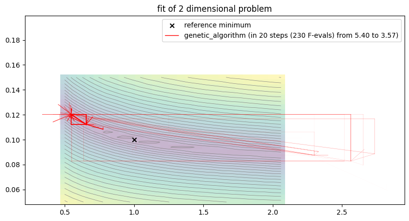
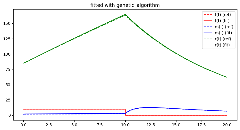
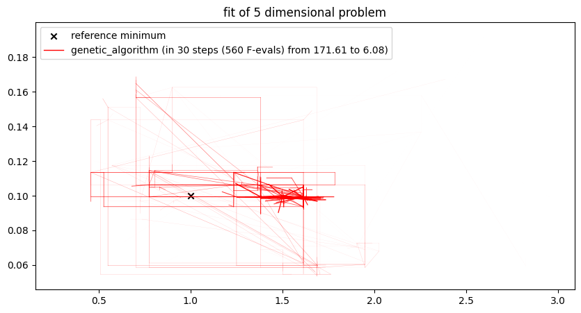
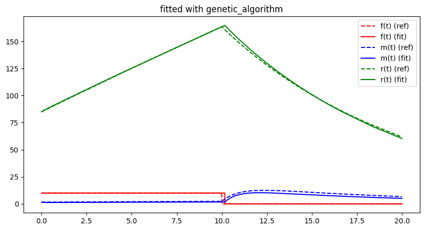
Particle Swarm Optimisation
The Particle Swarm Optimisation (PSO) is another highly applied population-based method to compute optima for non-differentiable functions. Different to the Genetic Algorithm it is much more strictly defined and uses a much fewer number of hyperparameters. In this strategy, every indiviudal from the population is regarded as a member of a swarm and its parametrisation is interpreted as its current position in the swarm. Instead of creating new individuals as in the Genetic Algorithm, the population update consists of updating the individual positions based on an movement-inspired update law.
Movement is always related to velocities. Therefore, in addtion to an initial position of the -th individual, an initial velocity must be defined. While the velocity must have the same vector-dimension as the parameter itself, it does not need to be part of the parameter space . Setting is a legitimate choice.
Clearly, positions are updated by applying the classic movement law
whereas , again, stands for some function which makes sure that the parameter space is not left. We furthermore define the update of the velocity.
Let refer to the parameters for the -th individual at algorithm step , then define
The two quantities represent the “best” place at which the individual or the total swarm, respectively, have ever visited over the course of the iteration. They are henceforth called the personal-optimum and the swarm optimum. The update concept of the particle swarm otimization considers that every individual is somewhat attacted to these two poins, i.e. that the velocity update incorporates the two components and . It is computed by
In this formula, represent two distributed random numbers and are scalar hyperparameters.
| Hyperparameter | Symbol | Range/Space | Considerations |
|---|---|---|---|
| Size of the population | integer greater than 1 | Reasonable sizes depend on the dimension of the problem. In most cases values between 20 and 200 are used. | |
| Distribution of initial individuals | - | some mapping | In most implementations, the initial individuals is drawn uniformly from the parameter space. However, also a more homogeneous mapping is possible using deterministic space-filling sequencese, such as the Sobol sequence Sobol’ (1967) |
| Parameters for the velocity components | Need to be tuned properly for getting a good convergence behaviour. In the best case the swarm describes a vortex with decreasing radius. Parameter consitutes the inertia of the individual. I.e. chosing a larger value will slow down the convergence speed allowing for more parameter space exploration. In general, choosing the three values too large will cause unwanted oscillations. Manually cutting the speed by a max-velocity parameter can help. | ||
| Parameter space mapping | with | Could be if the parameter space is unbounded or no bounds are known. Otherwise, it should map any potential modified individual outside the parameter-space back into the parameterspace. |
Experiment: Lithium-Cluster Dynamics (Particle Swarm Optimisation)
The algorithm can be directly applied without addtional adaptation.
class ParticleSwarmOptimizer(PopulationBasedOptimizer):
    def __init__(
        self,
        function: Callable[[np.ndarray], float] | None,
        parameter_space: np.ndarray,
        pop_size: int = 50,
        omega: float = 0.1,
        phi: float = 0.1,
        psi: float = 0.1,
    ) -> None:
        """Optimizer using Particle Swarm Optimization
        :param function: callable function to minimize. Can be None and specified later
        :param parameter_space: boudaries of the parameter space
        :param pop_size: size of the population
        :param omega: inertia parameter for the current velocity
        :param phi: attraction to the personal optimum
        :param psi: attraction to the swarm optimum
        """
        super().__init__(function, "particle_swarm_optmisation", parameter_space)
        self.pop_size = pop_size
        self.omega = omega
        self.phi = phi
        self.psi = psi
        self.velocities: list[np.ndarray] = None

    def create_population(self) -> tuple[list[np.ndarray], list[float | None]]:
        """Creates the initial population using the Sobol sequence.
        Initializes the velocities with zero-vectors
        :return: created population and corresponding function values (all None)
        """
        dim = len(self.parameter_space_lb)
        sampler = qmc.Sobol(d=dim, scramble=False)
        sample = sampler.random_base2(int(np.log2(self.pop_size) + 1))
        pop = [
            self.parameter_space_lb + sample[i, :] * self.parameter_diff
            for i in range(self.pop_size)
        ]
        self.velocities = [np.zeros(dim) for k in range(self.pop_size)]
        self.personal_opt = [(None, None) for k in range(self.pop_size)]
        self.swarm_opt = (None, None)
        return pop, [None for p in pop]

    def update_population(
        self, pop: list[np.ndarray], fpop: list[float]
    ) -> tuple[list[np.ndarray], list[float | None]]:
        """Performs a full update step for the population.
        I.e. updates the velocities and adds them to the population.
        :param pop: current population
        :param fpop: corresponding function values
        :return: updated population and correspondng function values (None for all in this algorithm)
        """
        for k, (p, fp) in enumerate(zip(pop, fpop)):
            if self.personal_opt[k][0] is None or fp < self.personal_opt[k][1]:
                self.personal_opt[k] = (p, fp)
                if self.swarm_opt[0] is None or fp < self.swarm_opt[1]:
                    self.swarm_opt = (p, fp)
        # update velocity and positions
        pop_new = list()
        for k, p in enumerate(pop):
            x1 = self.omega * self.velocities[k]
            x2 = self.phi * (self.personal_opt[k][0] - p)
            x3 = self.psi * (self.swarm_opt[0] - p)
            self.velocities[k] = x1 + np.random.random() * x2 + np.random.random() * x3
            p_new = self.map_to_parameterspace(p + self.velocities[k])
            self.segments[self.step].append((p, p_new))
            pop_new.append(p_new)
        return pop_new, [None for x in pop_new]


np.random.seed(12346)
free_parameter_indices = np.array([0, 1])
pso_opt = ParticleSwarmOptimizer(
    None,
    parameter_space=extract_free_parameter_space(free_parameter_indices),
    pop_size=20,
    omega=0.7,
    phi=0.4,
    psi=0.4,
)
run_lithium_cluster_test(pso_opt, free_parameter_indices, 15)
free_parameter_indices = np.array([0, 1, 2, 3, 6])
pso_opt = ParticleSwarmOptimizer(
    None,
    parameter_space=extract_free_parameter_space(free_parameter_indices),
    pop_size=30,
    omega=0.7,
    phi=0.5,
    psi=0.5,
)
run_lithium_cluster_test(pso_opt, free_parameter_indices, 30)
plt.show()
##### Start fitting of 2 dimensional problem with PARTICLE_SWARM_OPTMISATION ####
step 0: best individual is [2.3 0.0875] with min error 5.399165100320637, max error 3698.4935142057034
step 1: best individual is [2.3 0.0875] with min error 5.399165100320637, max error 3571.5923539525293
step 2: best individual is [1.35862964 0.09310339] with min error 3.6731400063487403, max error 2379.9983052532893
step 3: best individual is [1.7658316 0.09067957] with min error 4.44464294278783, max error 1409.2402249934864
step 4: best individual is [1.53886579 0.09028884] with min error 4.564643629843429, max error 307.2739306444821
step 5: best individual is [1.58145235 0.09177707] with min error 3.7403221672648543, max error 298.34853867482053
step 6: best individual is [1.5791518 0.09179076] with min error 3.7361968081651744, max error 124.82213741650857
step 7: best individual is [1.36322033 0.09336778] with min error 3.526419248629488, max error 246.0596471554554
step 8: best individual is [1.23845499 0.09690945] with min error 3.651925004761451, max error 261.0578088922912
step 9: best individual is [1.06643308 0.09938785] with min error 3.1672591259050105, max error 141.31439686540116
step 10: best individual is [0.94601774 0.10112273] with min error 3.1558111147265384, max error 71.17147921217926
step 11: best individual is [1.13278475 0.09704508] with min error 3.277692650272135, max error 38.816777795011134
step 12: best individual is [1.03121966 0.10034527] with min error 3.207620618438773, max error 58.8356833819121
step 13: best individual is [1.07595239 0.09879682] with min error 3.0972285302714138, max error 43.631945479758194
step 14: best individual is [1.01247012 0.10010199] with min error 3.077132789785011, max error 26.413328522149325
step 15: best individual is [0.98759533 0.10043046] with min error 3.09158312399778, max error 16.07969232288382
Summary: steps 15, func-evals: 320, accuracy x: 0.013130326495815707, residual: 3.09158312399778
##### Start fitting of 5 dimensional problem with PARTICLE_SWARM_OPTMISATION ####
step 0: best individual is [ 1.25 0.10625 0.12875 2.6625 10.625 ] with min error 171.60582264641923, max error 29129.164666452518
step 1: best individual is [ 1.25 0.10625 0.12875 2.6625 10.625 ] with min error 171.60582264641923, max error 25328.600065018778
step 2: best individual is [ 1.38607092 0.11353951 0.11951662 2.26886625 11.35395138] with min error 104.78677136006905, max error 9308.973355946939
step 3: best individual is [ 1.31047885 0.10948994 0.12464608 2.48754332 10.94899385] with min error 57.669116190579516, max error 1547.388123001476
step 4: best individual is [ 1.40738976 0.11138749 0.10555237 2.44436969 10.479927 ] with min error 26.036872043121477, max error 2341.7801155705997
step 5: best individual is [ 1.18113873 0.12293669 0.10454076 2.52769254 10.07416074] with min error 22.462854517203535, max error 3636.369423263105
step 6: best individual is [ 1.27839916 0.11619214 0.10766351 2.49156405 10.36961176] with min error 23.43960099641212, max error 1990.4758718568612
step 7: best individual is [ 1.25062995 0.11987454 0.10794584 2.45384068 10.41838972] with min error 24.669427784444313, max error 431.0128874055634
step 8: best individual is [ 1.22037453 0.12020376 0.10645044 2.49504801 10.31862039] with min error 21.780765571034227, max error 2349.4757263121455
step 9: best individual is [1.26104116 0.12058353 0.09787566 2.50949846 9.98250678] with min error 20.588155084562345, max error 2123.9773760721678
step 10: best individual is [ 1.22674532 0.12088551 0.10345371 2.50689391 10.15050632] with min error 20.20563201672335, max error 1080.1908590081287
step 11: best individual is [ 1.23825171 0.12044802 0.1027777 2.50811225 10.17805489] with min error 20.123567193409443, max error 206.37278165325955
step 12: best individual is [ 1.23956343 0.12088195 0.10172554 2.50159803 10.09502122] with min error 20.023376015702503, max error 380.10510136537266
step 13: best individual is [ 1.23957337 0.12076387 0.1017777 2.50491324 10.10381767] with min error 20.020965078045666, max error 447.35020576524425
step 14: best individual is [ 1.23781268 0.12006285 0.10249452 2.50076231 10.16919737] with min error 19.9876354370058, max error 304.5341123136253
step 15: best individual is [ 1.23898358 0.12045888 0.101979 2.50089621 10.1438519 ] with min error 20.03146640310554, max error 113.63221860013178
step 16: best individual is [ 1.23751359 0.1201195 0.10238679 2.5013412 10.14704849] with min error 19.971035009727245, max error 109.63446419516386
step 17: best individual is [ 1.24573904 0.12063644 0.10149732 2.48763548 10.07254186] with min error 19.996475713197853, max error 96.65191397626711
step 18: best individual is [ 1.23011974 0.12060444 0.10268376 2.4995212 10.13157488] with min error 19.960601752733446, max error 133.49312220289121
step 19: best individual is [ 1.23601413 0.12051173 0.10182615 2.49689505 10.13579967] with min error 19.9793290707561, max error 63.1251687092746
step 20: best individual is [ 1.23268666 0.12065947 0.10224623 2.49302424 10.14560755] with min error 19.912009477560034, max error 46.886413032914945
step 21: best individual is [ 1.23356226 0.12079728 0.10203212 2.49364632 10.12856924] with min error 19.896699705535493, max error 41.892027496796935
step 22: best individual is [ 1.2305388 0.12080586 0.10248748 2.49041114 10.1477632 ] with min error 19.89996952553506, max error 60.74506148010751
step 23: best individual is [ 1.23012661 0.12081796 0.10275364 2.49432389 10.14643032] with min error 19.901661472671282, max error 28.714082837804202
step 24: best individual is [ 1.22755208 0.12097812 0.10312514 2.49255569 10.15428292] with min error 19.869082648316187, max error 26.486862932352356
step 25: best individual is [ 1.23197757 0.12089015 0.10232648 2.4925898 10.13639523] with min error 19.84649940580932, max error 26.922289553607573
step 26: best individual is [ 1.23015962 0.12077367 0.10254452 2.49386342 10.13869184] with min error 19.86683302644345, max error 26.851056595647698
step 27: best individual is [ 1.23013315 0.1208559 0.10260674 2.49103817 10.14864434] with min error 19.865388065246357, max error 24.673844127276322
step 28: best individual is [ 1.22861581 0.12085485 0.10268836 2.49036902 10.14690858] with min error 19.877275611046965, max error 23.008657748823026
step 29: best individual is [ 1.23122529 0.12049128 0.10206304 2.49352959 10.13989968] with min error 19.876116274676875, max error 20.75130043231014
step 30: best individual is [ 1.23361958  0.12063295  0.10262248  2.490131   10.1327217 ] with min error 19.82472287835384, max error 22.939432687708585
Summary: steps 30, func-evals: 930, accuracy x: 1.5226635480032933, residual: 19.82472287835384
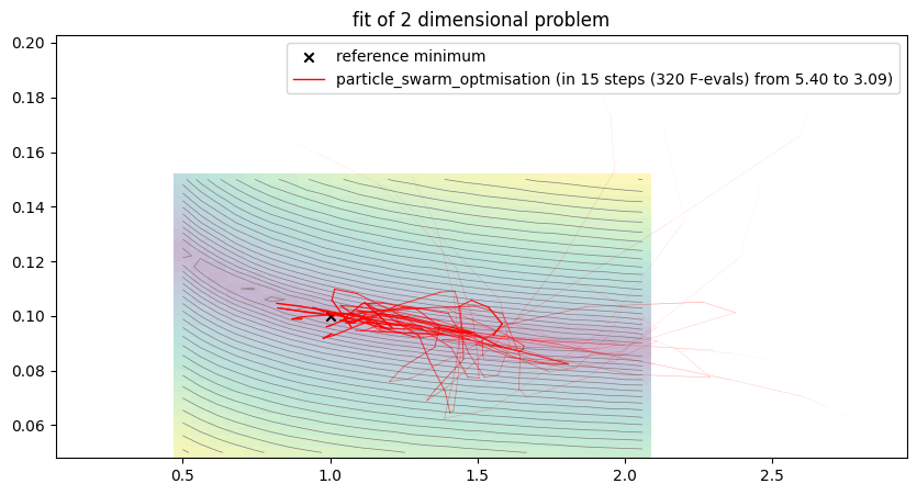
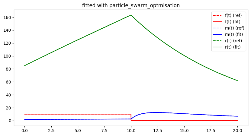
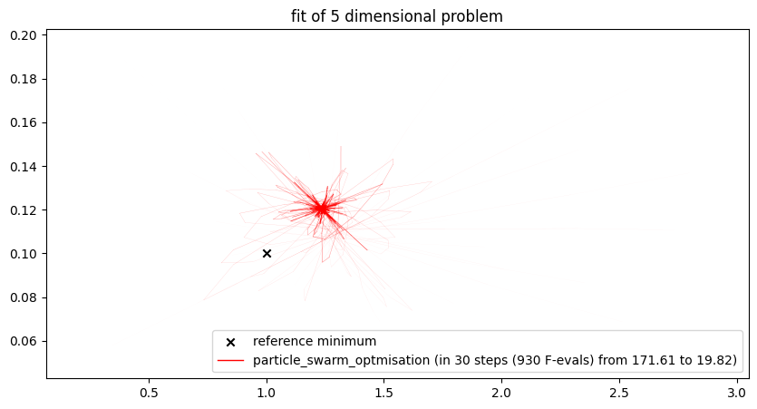
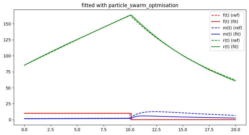
Due to their high number of hyperparameters, out-of-the box implementations of metaheuristics usually quite large and complicated to use. Examples for genetic algorithms in Python are [PyGAD}(https://
Downhill-Simplex Method
The Downhill-Simplex Method (see, Nelder & Mead (1965)) is a highly creative method based on so calles simplices, i.e. triandles in 2D or tetraeder in 3D. For an arbitrary dimension it is defined by corner points forming an object with sides.
The state of the algorithm is always a simplex in the parameter space. That means we will describe the algorithm using the notation of a population-based metaheuristic with a constant population size of . The core idea of the method is now to modify the simplex at each step so that it gradually contracts towards the optimum. This means that it must first move in such a way that the optimum lies inside the simplex, and then shrink towards it.
In each update step, the control points are first sorted by their fitness; that is, let denotes the corner point prior to the -th algorithm step that yields the smallest function value , and corresponds to the corner point with the largest. In the update step, the algorithm first aims to improve the performance of , by attempting a couple of alternatives. For this purpose, it computes the centre-point of the opposing hyperplane , and examines points along the line
These are the
reflected point with and function value ,
expanded point with and function value ,
outward-contracted point with and function value ,
inward-contracted point with and function value . We refer to the sketch below for a visual interpretation of these points. Dependent on the found function values either of the four replaces for the next algorithm step. I.e.
However, there is one last remaining alternative, that the simplex shrinks entirely. In this case, all points with the exception of , are moved towards . I.e.
with some positive . Note, that any step is usually cut at the borders of the parameter space to make sure the solution is in bounds.

| Hyperparameter | Symbol | Range/Space | Considerations |
|---|---|---|---|
| Position of initial simplex | - | some mapping | Should be big enough to cover a large part of the parameter space. |
| Parameters for computing the points and the shrinking behaviour | were the default parameters by Nelder and Mead and still work nicely. |
Experiment: Lithium-Cluster Dynamics (Downhill Simplex)
The method can be applied without adaption.
class DonwhillSimplexOptimizer(PopulationBasedOptimizer):
    def __init__(
        self,
        function: Callable[[np.ndarray], float],
        parameter_space: np.ndarray,
        alpha=1.0,
        beta=0.5,
        gamma=2.0,
        rho=-0.5,
        sigma=0.5,
    ) -> None:
        """Implementation of the Downhill Simplex Method by Nelder and Mead
        :param function: function to minimize, can be None to be set later on
        :param parameter_space: parameter boundaries
        :param alpha: reflected point parameter
        :param beta: inwards contracted point parameter
        :param gamma: expanded point parameter
        :param rho: outwards contracted point parameter
        :param sigma: shrinking parameter
        """
        super().__init__(function, "downhill_simplex", parameter_space)
        self.pop_size = len(self.parameter_space_lb) + 1
        self.alpha = alpha
        self.beta = beta
        self.gamma = gamma
        self.rho = rho
        self.sigma = sigma

    def add_simplex_segments(self, pop: list[np.ndarray]) -> None:
        """Helper method to plot the simplices.
        The probleme here is that in n-D with n>2 the projecion of a simpex into the 2-D plane is not a triangle. So we use the convex hull.
        :param pop: current simplex vetices
        :return:
        """
        points = np.array([x[:2] for x in pop])
        hull = spatial.ConvexHull(points)
        for simplex in hull.simplices:
            self.segments[self.step].append(
                (points[simplex[0], :], points[simplex[1], :])
            )

    def create_population(self) -> tuple[list[np.ndarray], list[float | None]]:
        """Creates the initial simplex which spans nicely over the parameter space.
        We use N+1 of the 2^N vertices of the 2^N corners of the N-D hyper-cube [lb+0.3(ub-lb),lb+0.7*(ub-lb)] whereas lb and ub refer to the boundaries of the parameter-space.
        :return: initial vertices and corresponding function values (will all be None here)
        """
        pop = list()
        low = self.parameter_space_lb + 0.3 * (
            self.parameter_space_up - self.parameter_space_lb
        )
        upp = self.parameter_space_lb + 0.7 * (
            self.parameter_space_up - self.parameter_space_lb
        )
        for i in range(self.pop_size - 1):
            p = low.copy()
            p[i] = upp[i]
            pop.append(p)
        pop.append(low.copy())
        return pop, [None for p in pop]

    def shrink(self, pop_sorted: list[np.ndarray]) -> list[np.ndarray]:
        """Shrinks the simplex towards its first vertex.
        I.e. the resulting list will have the same first entry as the input, but all others are shifted towards it.
        :param pop_sorted: sorted list of vertices
        :return: list of vertices shrunk to the first vertex
        """
        pop_new = [pop_sorted[0]]
        for p in pop_sorted[1:]:
            pop_new.append(p + self.sigma * (pop_sorted[0] - p))
        return pop_new

    def update_population(
        self, pop: list[np.ndarray], fpop: list[float]
    ) -> tuple[list[np.ndarray], list[float | None]]:
        """Updates the vertices of the simplex according to the rules by Nelder and Mead
        :param pop: current vertices
        :param fpop: corresponding function values
        :return: updated vertices and corresponding function values (depending on the update, either one or pop_size-1 of those are None)
        """
        # join the two and sort
        pop_and_f = [(p, fp) for p, fp in zip(pop, fpop)]
        pop_and_f.sort(key=lambda x: x[1])
        # split them up again
        pop_new = [x[0] for x in pop_and_f]
        fpop_new = [x[1] for x in pop_and_f]
        # compute candidates and start with if-else stuff
        p0 = 1 / (self.pop_size - 1) * sum(pop_new[:-1])
        pr = p0 + self.alpha * (pop_new[-1] - p0)  # reflected point
        fr = self.function(pr)
        if fr >= fpop_new[-1]:  # we made it worse..
            pci = p0 + self.beta * (pop_new[-1] - p0)  # inwards contracted point
            fci = self.function(pci)
            if fci > fpop_new[-1]:
                pop_new = self.shrink(pop_new)
                fpop_new = [fpop_new[0], *[None for x in range(self.pop_size - 1)]]
            else:
                pop_new[-1] = pci
                fpop_new[-1] = fci
        elif fr >= fpop_new[-2]:  # we made it a little bit better..
            pco = p0 + self.rho * (pop_new[-1] - p0)
            fco = self.function(pco)  # outwards contracted point
            if fco > fr:
                pop_new = self.shrink(pop_new)
                fpop_new = [fpop_new[0], *[None for x in range(self.pop_size - 1)]]
            else:
                pop_new[-1] = pco
                fpop_new[-1] = fco
        elif fr >= fpop_new[0]:  # we made it a lot better..
            pop_new[-1] = pr
            fpop_new[-1] = fr
        else:  # there might be even more potential...
            pe = p0 + self.gamma * (pop_new[-1] - p0)  # expanded point
            fe = self.function(pe)
            if fe > fr:
                pop_new[-1] = pr
                fpop_new[-1] = fr
            else:
                pop_new[-1] = pe
                fpop_new[-1] = fe
        self.add_simplex_segments(pop_new)
        return pop_new, fpop_new


np.random.seed(12346)
free_parameter_indices = np.array([0, 1])
simplex_opt = DonwhillSimplexOptimizer(
    None, parameter_space=extract_free_parameter_space(free_parameter_indices)
)
run_lithium_cluster_test(simplex_opt, free_parameter_indices, 15)
free_parameter_indices = np.array([0, 1, 2, 3, 6])
simplex_opt = DonwhillSimplexOptimizer(
    None, parameter_space=extract_free_parameter_space(free_parameter_indices)
)
run_lithium_cluster_test(simplex_opt, free_parameter_indices, 30)
plt.show()
##### Start fitting of 2 dimensional problem with DOWNHILL_SIMPLEX ####
step 0: best individual is [1.04 0.095] with min error 8.624128390200285, max error 875.5788426326797
step 1: best individual is [1.04 0.095] with min error 8.624128390200285, max error 289.52691514013947
step 2: best individual is [1.04  0.095] with min error 8.624128390200285, max error 97.01719140196576
step 3: best individual is [1.04  0.095] with min error 8.624128390200285, max error 39.139699445216856
step 4: best individual is [1.04  0.095] with min error 8.624128390200285, max error 25.339230053451647
step 5: best individual is [1.04  0.095] with min error 8.624128390200285, max error 20.39855008709943
step 6: best individual is [1.04  0.095] with min error 8.624128390200285, max error 14.720517751242092
step 7: best individual is [1.49445312 0.09599609] with min error 7.890299003177961, max error 10.262207893628705
step 8: best individual is [1.37126953 0.09630371] with min error 5.333658377082567, max error 8.624128390200285
step 9: best individual is [1.23643066 0.09557495] with min error 3.2673947354173905, max error 7.890299003177961
step 10: best individual is [1.23643066 0.09557495] with min error 3.2673947354173905, max error 5.469537940947211
step 11: best individual is [1.23643066 0.09557495] with min error 3.2673947354173905, max error 5.333658377082567
step 12: best individual is [1.23643066 0.09557495] with min error 3.2673947354173905, max error 4.499848195841691
step 13: best individual is [1.23643066 0.09557495] with min error 3.2673947354173905, max error 4.329285704919789
step 14: best individual is [1.23643066 0.09557495] with min error 3.2673947354173905, max error 3.922266151455132
step 15: best individual is [1.23643066 0.09557495] with min error 3.2673947354173905, max error 3.7525021253165423
Summary: steps 15, func-evals: 33, accuracy x: 0.24053599444192086, residual: 3.2673947354173905
##### Start fitting of 5 dimensional problem with DOWNHILL_SIMPLEX ####
step 0: best individual is [1.04  0.095 0.067 1.11  9.5  ] with min error 72.97854239340066, max error 3295.8581819604433
step 1: best individual is [1.04  0.095 0.067 1.11  9.5  ] with min error 72.97854239340066, max error 1299.6365476220458
step 2: best individual is [1.04  0.095 0.067 1.11  9.5  ] with min error 72.97854239340066, max error 1200.1150128475872
step 3: best individual is [1.04  0.095 0.067 1.11  9.5  ] with min error 72.97854239340066, max error 448.17049453829907
step 4: best individual is [1.182352  0.098666  0.1070596 1.247268  9.683    ] with min error 50.74709575642339, max error 404.6351727913976
step 5: best individual is [1.182352  0.098666  0.1070596 1.247268  9.683    ] with min error 50.74709575642339, max error 350.2748679409687
step 6: best individual is [1.182352  0.098666  0.1070596 1.247268  9.683    ] with min error 50.74709575642339, max error 168.446171695679
step 7: best individual is [1.182352  0.098666  0.1070596 1.247268  9.683    ] with min error 50.74709575642339, max error 152.11415036921906
step 8: best individual is [1.182352  0.098666  0.1070596 1.247268  9.683    ] with min error 50.74709575642339, max error 138.36544179188684
step 9: best individual is [1.182352  0.098666  0.1070596 1.247268  9.683    ] with min error 50.74709575642339, max error 110.90529343587183
step 10: best individual is [1.182352  0.098666  0.1070596 1.247268  9.683    ] with min error 50.74709575642339, max error 85.64708082853176
step 11: best individual is [1.182352  0.098666  0.1070596 1.247268  9.683    ] with min error 50.74709575642339, max error 84.4403094482692
step 12: best individual is [1.25364524 0.10072196 0.07868041 1.35690385 9.72176236] with min error 45.91008943532916, max error 72.97854239340066
step 13: best individual is [1.14857627 0.09679151 0.07493984 1.25967622 9.6136921 ] with min error 42.92670515948754, max error 63.18778824898992
step 14: best individual is [1.24756784 0.09855307 0.08018564 1.38555015 9.81092272] with min error 36.27618301648533, max error 52.64383694645794
step 15: best individual is [1.20770815 0.09766624 0.07862345 1.52356557 9.65104978] with min error 34.495932015537, max error 51.11069011615025
step 16: best individual is [1.31676154 0.0981056  0.08035826 1.33859209 9.68009329] with min error 32.29741388633453, max error 50.74709575642339
step 17: best individual is [1.2086019  0.09851684 0.09280856 1.31006279 9.68925202] with min error 15.92081793471191, max error 45.91008943532916
step 18: best individual is [1.2086019  0.09851684 0.09280856 1.31006279 9.68925202] with min error 15.92081793471191, max error 42.92670515948754
step 19: best individual is [1.2086019  0.09851684 0.09280856 1.31006279 9.68925202] with min error 15.92081793471191, max error 36.27618301648533
step 20: best individual is [1.2086019  0.09851684 0.09280856 1.31006279 9.68925202] with min error 15.92081793471191, max error 34.495932015537
step 21: best individual is [1.2086019  0.09851684 0.09280856 1.31006279 9.68925202] with min error 15.92081793471191, max error 33.993074859984574
step 22: best individual is [1.2086019  0.09851684 0.09280856 1.31006279 9.68925202] with min error 15.92081793471191, max error 32.79646679526627
step 23: best individual is [1.2086019  0.09851684 0.09280856 1.31006279 9.68925202] with min error 15.92081793471191, max error 32.29741388633453
step 24: best individual is [1.2086019  0.09851684 0.09280856 1.31006279 9.68925202] with min error 15.92081793471191, max error 29.715736146650052
step 25: best individual is [1.2086019  0.09851684 0.09280856 1.31006279 9.68925202] with min error 15.92081793471191, max error 28.849939589160584
step 26: best individual is [1.2086019  0.09851684 0.09280856 1.31006279 9.68925202] with min error 15.92081793471191, max error 27.84425908570139
step 27: best individual is [1.2086019  0.09851684 0.09280856 1.31006279 9.68925202] with min error 15.92081793471191, max error 27.28755500208592
step 28: best individual is [1.2086019  0.09851684 0.09280856 1.31006279 9.68925202] with min error 15.92081793471191, max error 26.3224829571317
step 29: best individual is [1.2086019  0.09851684 0.09280856 1.31006279 9.68925202] with min error 15.92081793471191, max error 25.190828750657005
step 30: best individual is [1.2086019  0.09851684 0.09280856 1.31006279 9.68925202] with min error 15.92081793471191, max error 24.615873227376557
Summary: steps 30, func-evals: 66, accuracy x: 0.3821138412676784, residual: 15.92081793471191
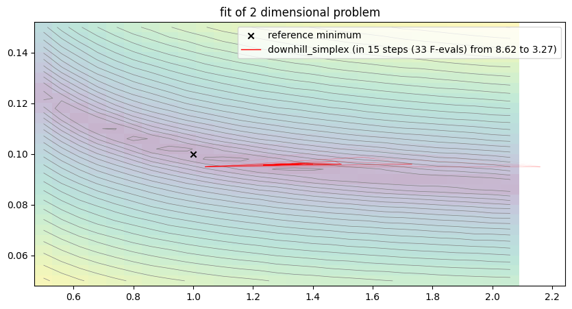
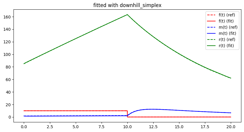
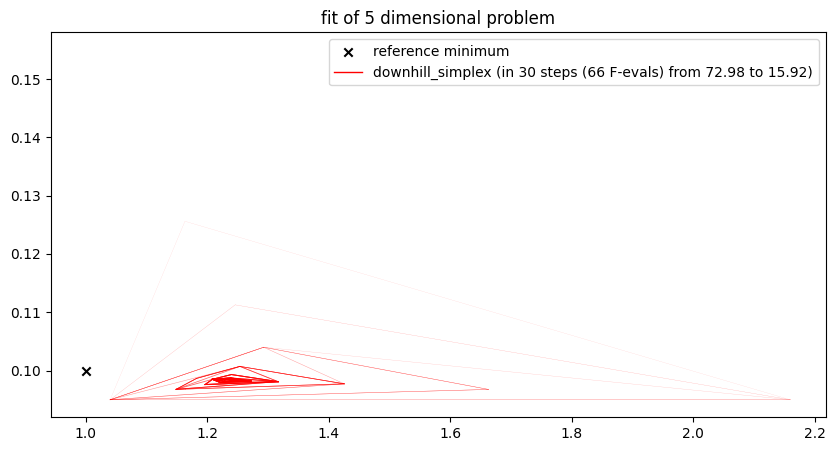
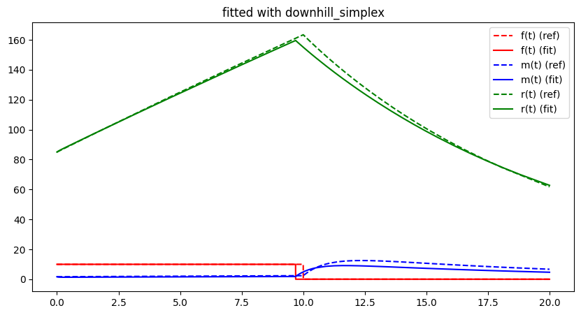
Also the more “genetic” Python package scipy offers implementations of methods which do not require computation of a gradient. Besides the mentioned Donwhill Simplex Method (minimize with method="Nelder-Mead") we would also like to emphasise the quite successfull Powell Algorithm (minimize with method="Powell").
bfgs_opt = SciPyOptimizer(None, "Nelder-Mead")
cg_opt = SciPyOptimizer(None, "Powell")
run_lithium_cluster_test([bfgs_opt, cg_opt], np.array([0, 1]), [0, 0])
run_lithium_cluster_test([bfgs_opt, cg_opt], np.array([0, 1, 2, 3, 6]), [0, 0])
plt.show()
##### Start fitting of 2 dimensional problem with SCIPY-NELDER-MEAD ####
step 0: [1.6 0.125] -> 370.6116275091885
step 69: [1.01828528 0.09990318] -> 3.0378379590496056
Summary: steps 69, func-evals: 183, accuracy x: 0.018310900011124065, residual: 3.0378379590496056
##### Start fitting of 2 dimensional problem with SCIPY-POWELL ####
step 0: [1.6   0.125] -> 370.6116275091885
step 6: [0.75756256 0.10790434] -> 3.2524797140081563
Summary: steps 6, func-evals: 340, accuracy x: 0.2549975797610555, residual: 3.2524797140081563
##### Start fitting of 5 dimensional problem with SCIPY-NELDER-MEAD ####
step 0: [ 1.6    0.125  0.105  1.65  12.5  ] -> 1612.6191361568735
step 123: [ 1.92689959  0.0975862   0.11199648  1.76272856 10.30583618] -> 14.732703013122906
Summary: steps 123, func-evals: 271, accuracy x: 1.2069827088099012, residual: 14.732703013122906
##### Start fitting of 5 dimensional problem with SCIPY-POWELL ####
step 0: [ 1.6    0.125  0.105  1.65  12.5  ] -> 1612.6191361568735
step 11: [0.63602348 0.11294419 0.1006325  0.97273237 9.99836956] -> 3.3382224725814025
Summary: steps 11, func-evals: 1220, accuracy x: 0.38732115592696975, residual: 3.3382224725814025
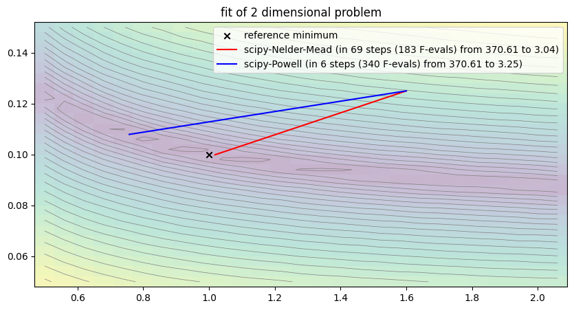
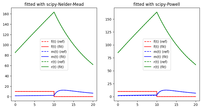
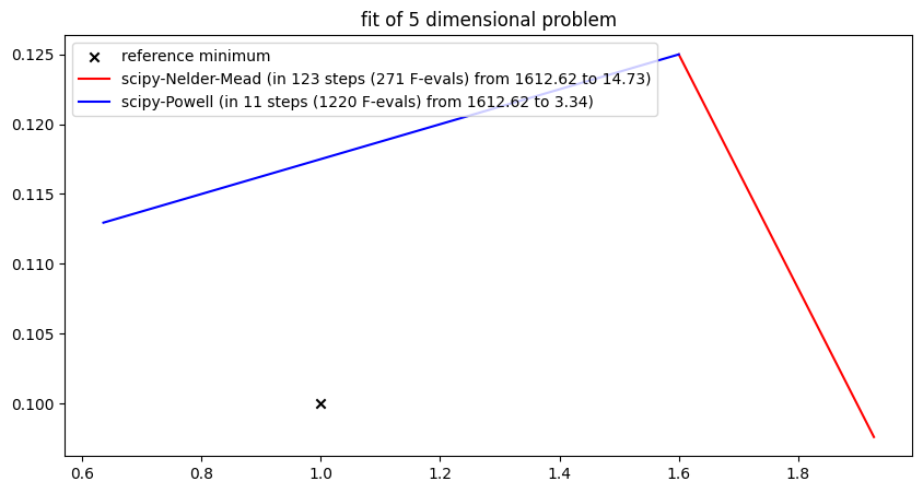
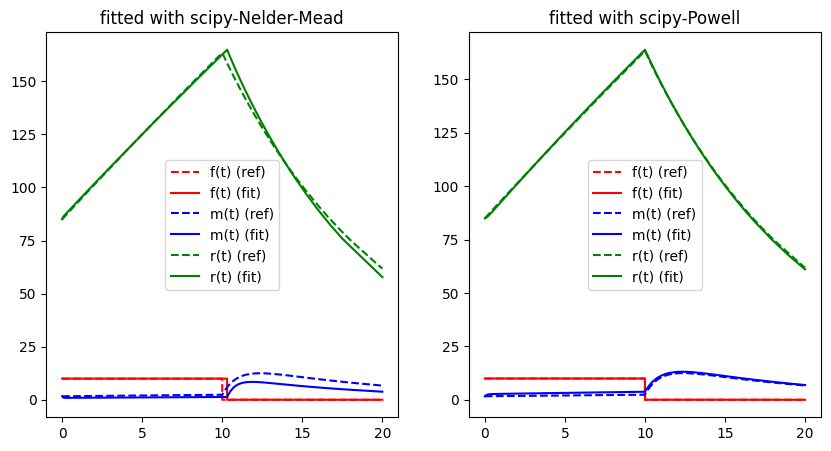
All presented algorithms have their pro’s and con’s. Gradient-based approaches converge extremely fast, but only if the problem is sufficiently well-defined. Metaheuristics require more tuning and have more hyperparameters to test. However, when configured properly, they can converger reliably to global optima. While a clear tradeoff between accuracy and function evaluations can be observed, the selection of the right method is more beneficial the giving the computer more time to compute, e.g. because it cannot get out of a local optimum. Eventually, there is no single best optimisation/calibration method (No Free Lunch, Wolpert et al. (1995)).
- Husinsky, W. (1991). Comparison 1: Lithium-Cluster Dynamics under Electron Bombardment - Definition. Simulation News Europe, 1(2).
- Head, J. D., & Zerner, M. C. (1985). A Broyden—Fletcher—Goldfarb—Shanno optimization procedure for molecular geometries. Chemical Physics Letters, 122(3), 264–270. 10.1016/0009-2614(85)80574-1
- Jamil, M., & Yang, X.-S. (2013). A literature survey of benchmark functions for global optimisation problems. International Journal of Mathematical Modelling and Numerical Optimisation, 4(2), 150–194.
- Polyak, B. T. (1969). The conjugate gradient method in extremal problems. USSR Computational Mathematics and Mathematical Physics, 9(4), 94–112. 10.1016/0041-5553(69)90035-4
- Blum, C., & Roli, A. (2003). Metaheuristics in combinatorial optimization: Overview and conceptual comparison. ACM Comput. Surv., 35(3), 268–308. 10.1145/937503.937505
- Bertsimas, D., & Tsitsiklis, J. (1993). Simulated Annealing. Statistical Science, 8(1). 10.1214/ss/1177011077
- Sobol, I. M. (1967). Distribution of points in a cube and approximate evaluation of integrals. USSR Computational Mathematics and Mathematical Physics, 7, 86–112.
- Sobol’, I. M. (1967). On the distribution of points in a cube and the approximate evaluation of integrals. USSR Computational Mathematics and Mathematical Physics, 7(4), 86–112. 10.1016/0041-5553(67)90144-9
- Nelder, J. A., & Mead, R. (1965). A simplex method for function minimization. The Computer Journal, 7(4), 308–313.
- Wolpert, D. H., Macready, W. G., & others. (1995). No free lunch theorems for search [Techreport]. Technical Report SFI-TR-95-02-010, Santa Fe Institute.