Pseudo Random Number Generation

In this chapter we present methods how a computer generates “random numbers”.

Objectives:

What is a Pseudo Random Number (PRN) and how are these numbers generated?
Which algorithms exists to create IID $U(0,1)$ distributed PRNs?
How do we decide which algorithm is better for which purpose?
How are IID $U(0,1)$ distributed PRNs transformed to arbitrary distributions?

from itertools import permutations

import math
import random
from abc import abstractmethod

import networkx
import numpy as np
import plotly.graph_objects as go
#%matplotlib ipympl
from matplotlib import pyplot as plt

from modelling_and_simulation_cookbook import Clock

Random Numbers¶

Many modelling approaches such as discrete event simulation or agent-based modelling make use of stochasticity. Stochasticity does not only allow the model to implement features which are perceived as random in the real system but also to depict its uncertainty.

In its most abstract form, the states/outputs of a conceptual stochastic model can be interpreted as a random variable $X:\Omega \rightarrow S$ , whereas $S$ is the set of all possible states of the model. The corresponding implemented model must then be able to compute specific observations $X(\omega)\in S$ of the random variable via simulation.

Case-Study: Coinflip¶

For example, $X=X_1+X_2$ , with $X_1,X_2\sim B(p)$ with $p=0.5$ is a feasible stochastic model for the total number of heads when flipping a coin twice. Hereby $B(p)$ refers to the Bernoulli distribution with probability $p$ , i.e. the random variable is 1 with probability $p$ and 0 otherwise. The outcome $X$ of the conceptual model is a function from the underlying probaility space $\Omega$ to the set $S$ of all possible outcomes, in this case, $S=\{0,1,2\}$ .

When implemented, the outcome must be made specific in terms of explicitly computing observations of the random number. I.e. the implemented model must compute two independent observations of $B(p)$ distributed random numbers and add them together. Since

\forall i\in \{1,2\}: P(X_i=1)=p=P(U_i<p)

(1)

for random variables $U_i$ uniformly distributed on the interval $[0,1)$ , i.e. $U_i\sim U(0,1)$ , we may use observations from a uniform distribution to compute observations from a Bernoulli distribution: $X_i=1\Leftrightarrow U_i<p$ . As a result, the implemented model is able to simulate one evaluation $X(\omega)$ from two independent observations from a uniform distribution.

Below we find an implementation and exceution of this simple model. Clearly, one observation of $X(\omega)$ is meaningless, but sufficiently many $\{X(\omega_1),X(\omega_2),\dots\}$ give us insights into the underlying distribution of the actual random variable $X$ from the conceptual model.

class CoinFlipModel:
    def __init__(self, p: float = 0.5) -> None:
        """Creates a model for a (weighted) coin-flip
        :param p: optional, probability for heads
        """
        self.p = p

    def run(self, flips: int = 2) -> int:
        """Returns the number of heads after a number of flips
        :param flips: number of flips
        :return: number of heads
        """
        heads = 0
        for n in range(flips):
            if np.random.random() < self.p:
                heads += 1
        return heads


iters = 200
flips = 2
mdl = CoinFlipModel()
results = np.zeros(flips + 1)
for k in range(iters):
    x = mdl.run(flips)
    results[x] += 1
print(f"distribution for the number of heads after {flips} flips: {results / iters}")

distribution for the number of heads after 2 flips: [0.25 0.5  0.25]

Pseudo Random Number Generation - General Concept¶

Clearly, the simulation is fundamentally dependent on (a) the computer’s ability to perform the operation np.random.random which should return (an observation of) a $U(0,1)$ distributed random number and (b) the ability to transform the number to match the desired distribution, in this case, the Bernoulli distribution. These two steps are the general workflow for sampling from given distributions and there are a series of methods for them which we want to discuss in this notebook.

While process (b) mostly relies on mathematical transformations and numerical approximations, the true “magic” of random number generation happens in step (a). In principle, it possible to get actually random numbers by linking the computer to real-time processes which are considered to be random. Examples are random.org where random numbers are computed from real-time athmospheric noise measurements and Quantiki where similar things are done using quantum effects of photons. However, the main problems with these generators are not only the overhead time of connecting the computer with an actual experiment, but in particular the lack of reproducibility of experiments. It is a fundamental requirement for simulation models that results must be reproducible, firstly to ensure the transparency of the process, and secondly to support the validation and verification process. Yet actual random numbers are unique and lead to irreproducible outcomes.

As a result, simulations usually rely on so-called Pseudo Random Numbers (PRNs). In contrast to true random numbers, these number are computed using specifically designed algorithms. As a result, they are, by design, not truly random but only appear to be random - therefor pseudo random.

Generation of $U(0,1)$ PRNs¶

As described, the task here is to use algorithms to generate numbers that appear to be (1) uniformlydistributed over the interval $[0,1)$ , we write $X\sim U(0,1)$ , and (2) are independent and identically distributed (IID). Research into such methods has a long history that is still ongoing to this day. As applications become increasingly complex (e.g. in the fields of quantum computing or cryptography) and computer become more and more powerful, the requirements regarding how “random” the created numbers must seem are also rising. We must require that more and more effort must be put into detecting that a created number sequence only appears random but is not.

Midsquare Method¶

The midsquare method developed in the 1945 by John Von Neumann and Nicholas Metropolis (Von Neumann & others (1963)) shows that implementation of such methods is not as easy as it seems. The method is initialised (seeded) with a 4-digit integer $x$ . Squaring the number leads an 8-digit integer (pad with zeros if it is smaller) of which the middle 4 digits are taken for the update, i.e.

x_{i+1}=\lfloor x_i^2/100\rfloor \text{ mod } 10000.

(2)

The sequence

u_i=x_i/10000

(3)

should furthermore imitate a sequence of independent $U(0,1)$ distributed random numbers.

class RNG:
    def __init__(self):
        self.seed(12345)

    @abstractmethod
    def seed(self, seed: int) -> None:
        pass

    @abstractmethod
    def get_state(self) -> int:
        return 0

    @abstractmethod
    def draw(self) -> float:
        return 0.0


class MidSquareGenerator(RNG):
    """Implements the midsquare method by Von Neumann and Metropolis"""

    def seed(self, seed: int) -> None:
        self.z = seed

    def get_state(self) -> int:
        return self.z

    def draw(self) -> float:
        y = self.z**2
        mid = int(y / 100) % 10000
        self.z = mid
        return mid / 10000


gen = MidSquareGenerator()
seed = 7182
gen.seed(seed)
print(f"seed: {seed}")
for i in range(1000):
    v = gen.draw()
    print(f"{i + 1}: {v}")
    if v == 0.0:
        break

seed: 7182
1: 0.5811
2: 0.7677
3: 0.9363
4: 0.6657
5: 0.3156
6: 0.9603
7: 0.2176
8: 0.7349
9: 0.0078
10: 0.006
11: 0.0036
12: 0.0012
13: 0.0001
14: 0.0

At first, the methods seems to produce reliable results, however, it becomes quickly clear that the method has severe flaws (e.g. 0 is an absorbing steady-state of the sequence). Thus, while the method shows the key ideas of how PRNGs could work, smater methods are required.

General Iterative Concept¶

Alike the midsquare method $U(0,1)$ -PRNGs share the same internal structure which has three steps.

First, they are all initialised by an integer value, also called the seed. Using the same seed means getting the same number sequence. The seed is processed to compute the initial internal state $z$ of the generator

z_0=h(seed),

(4)

for some initialisation function $h$ . Usually the state is a single integer as well and $h=Id$ $, however it can become arbitrarily complex, such as a huge integer-vector for the Mersenne-Twister generator.

Second, whenever a RNG is drawn, the generator updates its internal state via a recursive update rule, i.e.

z_{i+1}=f(z_i),\quad \text{ or } \quad z_{i+1}=f(z_i,z_{i-1},\dots).

(5)

Modulus operations usually play a key role in this process.

Finally, an output function

u_{i+1}=g(z_{i+1})

(6)

is applied, mainly to norm the state to the interval $[0,1)$ .

Linear Congruential Generators¶

Linear Congruental Generators (LGC) first published in 1958 Thomson (1958) are likely the most famous class of PRNGs. A LGC is defined by

z_0=h(seed)=seed,\quad z_{i+1}=f(z_i)=(az_i+c)\text{ mod } m,\text{ and}\quad u_{i+1}=g(z_{i+1})=\frac{z_{i+1}}{m},

(7)

and three integer-valued parameters: a factor $a$ , an increment $c$ and a modulus $m$ . The three parameters define how well the generator works. In the example seen below, one parameterset works well while the other does not.

class LinearCongruentialGenerator(RNG):
    def __init__(self, a: int, c: int, m: int):
        super().__init__()
        self.a = a
        self.c = c
        self.m = m

    def seed(self, seed: int):
        self.z = seed

    def draw(self) -> float:
        self.z = (self.z * self.a + self.c) % self.m
        return self.z / self.m

    def get_state(self) -> int:
        return self.z


for params in [(5, 3, 64), (4, 2, 64)]:
    lcg = LinearCongruentialGenerator(*params)
    lcg.seed(12345)
    print(f"Parameters: {params}")
    for i in range(20):
        u = lcg.draw()
        z = lcg.get_state()
        print(f"u{i + 1}: {u:.04f}, z{i + 1}: {z}")

Parameters: (5, 3, 64)
u1: 0.5000, z1: 32
u2: 0.5469, z2: 35
u3: 0.7812, z3: 50
u4: 0.9531, z4: 61
u5: 0.8125, z5: 52
u6: 0.1094, z6: 7
u7: 0.5938, z7: 38
u8: 0.0156, z8: 1
u9: 0.1250, z9: 8
u10: 0.6719, z10: 43
u11: 0.4062, z11: 26
u12: 0.0781, z12: 5
u13: 0.4375, z13: 28
u14: 0.2344, z14: 15
u15: 0.2188, z15: 14
u16: 0.1406, z16: 9
u17: 0.7500, z17: 48
u18: 0.7969, z18: 51
u19: 0.0312, z19: 2
u20: 0.2031, z20: 13
Parameters: (4, 2, 64)
u1: 0.5938, z1: 38
u2: 0.4062, z2: 26
u3: 0.6562, z3: 42
u4: 0.6562, z4: 42
u5: 0.6562, z5: 42
u6: 0.6562, z6: 42
u7: 0.6562, z7: 42
u8: 0.6562, z8: 42
u9: 0.6562, z9: 42
u10: 0.6562, z10: 42
u11: 0.6562, z11: 42
u12: 0.6562, z12: 42
u13: 0.6562, z13: 42
u14: 0.6562, z14: 42
u15: 0.6562, z15: 42
u16: 0.6562, z16: 42
u17: 0.6562, z17: 42
u18: 0.6562, z18: 42
u19: 0.6562, z19: 42
u20: 0.6562, z20: 42

This behaviour is worth being analysed in more depth: The number of different values a LGC can produce is clearly limited by the value of $m$ . Since the modulus operation always returns a value between 0 and $m-1$ , a maximum of $m$ values can be created. As a direct consequence, at least after $m+1$ draws, the sequence will repeat itself, meaning that $m$ must be chosen considerably large in real applications. However, with unfortunate choices for $a, c$ and $m$ the sequence does not produce $m$ but only a smaller number of different values - the generator does not have full-period.

def compute_cycles(rng: LinearCongruentialGenerator):
    if rng.m > 2**11:
        print("too large m")
        return
    g = networkx.DiGraph()
    for i in range(rng.m):
        g.add_node(i)
    for i in range(rng.m):
        rng.seed(i)
        rng.draw()
        j = rng.get_state()
        g.add_edge(i, j)
    pos = networkx.spring_layout(g, seed=3)
    networkx.draw_networkx(g, pos)


paramss = [(5, 3, 16), (3, 3, 16), (5, 0, 16), (10, 1, 32), (15, 1, 32)]
for params in paramss:
    a = params[0]
    c = params[1]
    m = params[2]
    print(f"{a=}, {c=}, {m=}")
    lcg = LinearCongruentialGenerator(a, c, m)
    lcg.seed(0)
    sequence = list()
    sequence_u = list()
    for k in range(m):
        sequence_u.append(lcg.draw())
        sequence.append(lcg.get_state())
    print(sequence)
    plt.figure()
    compute_cycles(lcg)
    plt.title(f"{a=}, {c=}, {m=}")
plt.show()

a=5, c=3, m=16
[3, 2, 13, 4, 7, 6, 1, 8, 11, 10, 5, 12, 15, 14, 9, 0]

a=3, c=3, m=16
[3, 12, 7, 8, 11, 4, 15, 0, 3, 12, 7, 8, 11, 4, 15, 0]
a=5, c=0, m=16
[0, 0, 0, 0, 0, 0, 0, 0, 0, 0, 0, 0, 0, 0, 0, 0]

a=10, c=1, m=32
[1, 11, 15, 23, 7, 7, 7, 7, 7, 7, 7, 7, 7, 7, 7, 7, 7, 7, 7, 7, 7, 7, 7, 7, 7, 7, 7, 7, 7, 7, 7, 7]

a=15, c=1, m=32
[1, 16, 17, 0, 1, 16, 17, 0, 1, 16, 17, 0, 1, 16, 17, 0, 1, 16, 17, 0, 1, 16, 17, 0, 1, 16, 17, 0, 1, 16, 17, 0]

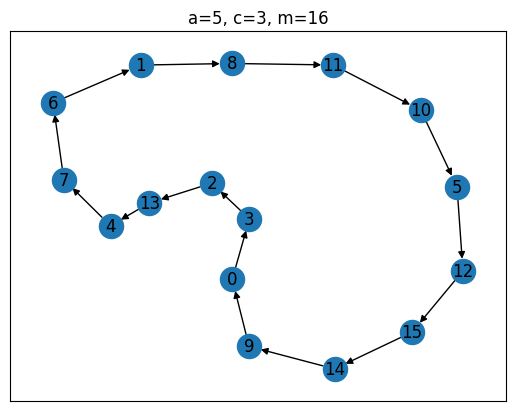
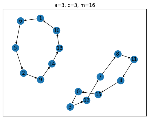
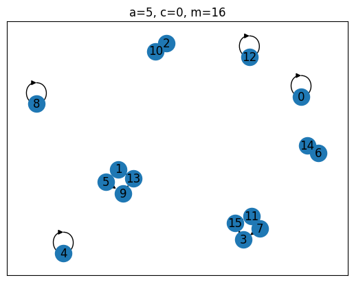
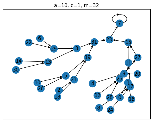
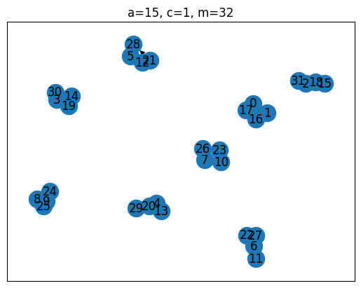
Of the four generators tested, the top one is clearly the best, as it has a ‘full period’, i.e. the sequence always cycles through all possible values between 0 and $m-1$ before repeating itself. The Full-Period Theorem by Hull and Dobell Hull & Dobell (1962) can be used to evaluate this up front. It states, that an LCG has full period iff

(a) $m$ and $c$ are coprime,
(b) $a-1$ is divisible by all prime factors of $m$ , and
(c) if $m$ is divisible by 4, then $a-1$ must be as well.

def has_full_period(
    rng: LinearCongruentialGenerator,
) -> tuple[bool, tuple[bool, bool, bool]]:
    # condition 1
    test1 = True
    gcd = math.gcd(rng.c, rng.m)
    if gcd != 1:
        test1 = False
    # create sieve of erathostenes and check condition 2
    test2 = True
    mx = int(rng.m**0.5)
    sieve = set(range(2, mx))
    for i in range(2, mx):
        if i in sieve:
            if (rng.m % i == 0) and ((rng.a - 1) % i != 0):
                test2 = False
                break
            rem = i
            while rem < mx:
                try:
                    sieve.remove(rem)
                except:
                    pass
                rem += i
    test3 = True
    if (rng.m % 4 == 0) and ((rng.a - 1) % 4 != 0):
        test3 = False
    all_tests = (test1, test2, test3)
    return all(all_tests), all_tests


for params in paramss:
    a = params[0]
    c = params[1]
    m = params[2]
    print(f"{a=}, {c=}, {m=}")
    lcg = LinearCongruentialGenerator(a, c, m)
    fp, conds = has_full_period(lcg)
    if fp:
        print("full period")
    else:
        abc = "abc"
        for i in range(3):
            if not conds[i]:
                print(f"condition {abc[i]} failed")

a=5, c=3, m=16
full period
a=3, c=3, m=16
condition c failed
a=5, c=0, m=16
condition a failed
a=10, c=1, m=32
condition b failed
condition c failed
a=15, c=1, m=32
condition c failed

Although a long period is measure of quality for a reliable LCG (or of a PRNG in general), it does not necessarily have to be “full”. Here is a table containing examples of LCGs that are actually used, or have been used, in software packages.

$m$	$a$	$c$	name/usage
2⁴⁸	25214903917	11	Math.random in Java (2025)
2³¹	214013	2531011	Legacy C Runtime PRNG / Windows (2025)
2³¹	$2^{16}+3$	0	RANDU, e.g. Fortran in the (60s-70s)
2³¹	69069	0	Marsaglia’s improved RANDU
$2^{31}-1$	7⁵	0	MINSTD, C++ standard library (2025), formally also used by Python

The bottom three generators are share $c=0$ by which they are counted to the subclass of multiplicative generators. By design these generators cannot have a full period and require properly chosen seed values (e.g. $seed=0$ is not reasonable).

Linear Congruential Generator Extensions¶

While LCGs are well-defined and easily understood PRNGs there is lots of room for improvement, in particular with respect to the statistical properties of the generated stream. Ideas, based on LCGs, include

Multiple Recursive Generators (MRG) with
$f(z_i,z_{i-1},...,z_{i-m}) = \sum_{j=0}^{m}a_jz_{i-j}\text{ mod } m$
(8)
Quadratic Congruential Generators (QCGs) with
$f(z_i) = az_i^2+bz_i+c \text{ mod } m$
(9)
Simultaneous Congruential Generators with $f^k(z_i^k)=a^kz_i^k+c^k\text{ mod } m^k$ for $k\in \{1,\dots,J\}$ and
$g=g(z_i^1,\dots,z_i^J)=\frac{1}{m}\left(\sum_{j=0}^{m}a_jz_{i-j}\text{ mod } m\right).$
(10)
Shuffled Generators, where $(z^1_j)_{j=1}^{m^2}=:\vec{z^1}$ is a sequence of $m^2$ numbers from generator 1 with modulus $m^1$ and $z_i^2$ is the current state of a second generator with modulus $m^2$ , then
$g(\vec{z^1},z_i^2)=\frac{1}{m_1}(\vec{z^1})_{z_i^2}.$
(11)

Mersenne-Twister¶

There are however also many ideas for generators beyond LCGs. The Mersenne-Twister Generator Matsumoto & Nishimura (1998) is the currently implemented PRNG in Python and uses a vector-valued state with 624 32-bit-integers. Whenever the generator should produce a new PRN it would process the $k$ -th index of this vector with several bit-wise operations and advance the state index $k$ by one. As soon as $k=624$ the state-vector is twisted by shifting the whole $624\cdot 32=19968$ -element bit-stream by 397 indices, i.e. the stream $(b_i)_{i=1}^{19968}$ is transformed to $b_i'=b_{i+397\text{ mod } 19968}$ . The resuling stream again can be interpreted as 624 entirely new integer numbers which have little-to-nothing to do with the original vector and $k$ can be set to 0 again.

random.seed(12345)
# getstate returns the current state of the rng
state = random.getstate()
# the first entry is simply a version id of the generator
print(f"version ID {state[0]}")
# the third entry is a cached value required e.g. to generate normally distributed PRNGs (we will not discuss this any deeper)
# the second entry, however, is the actual state of the generator.
print(f"state vector [{state[1][0]},{state[1][1]},...,{state[1][-2]}]")
# the last vector entry is the current vector index
print(f"k= {state[1][-1]}")
# this index always starts with 624 meaning that the generator will twist immidiately after seeding
print(random.random())  # call the RNG
state = random.getstate()
print(f"state vector [{state[1][0]},{state[1][1]},...,{state[1][-2]}]")
print(f"k= {state[1][-1]}")
print(random.random())  # call the RNG
state = random.getstate()
print(f"state vector [{state[1][0]},{state[1][1]},...,{state[1][-2]}]")
print(f"k= {state[1][-1]}")
print(random.random())  # call the RNG
random.setstate(state)  # set the state
print(random.random())  # call the RNG

version ID 3
state vector [2147483648,2105189241,...,238504783]
k= 624
0.41661987254534116
state vector [1060008160,340894186,...,229380103]
k= 2
0.010169169457068361
state vector [1060008160,340894186,...,229380103]
k= 4
0.8252065092537432
0.8252065092537432

It is interesing to observe that any call of the PRNG does not only shift the state vector by one but by two. This is due to the fact, that random.random creates 64-bit float values for which it requires two 32-bit integers. Finally, note that while it is possible to replicate the full stream by using the same seed, the Mersenne-Twister requires to set its full vector valued state to be set to some place “in the middle”.

Testing of PRNGs¶

Clearly not every PRNGs is eqally good w.r. to the properties of the resulting sequence. In general, the quality of a PRNG is measured by how difficult it is to proof that the generated random number stream is in fact not IID $U(0,1)$ . We distinguish between theoretical and empirical tests, whereas the prior use theoretical knowledge about the PRNG to derive certain properties and the latter statistically evaluate generated streams of PRNs. There are a by far less theoretical than empirical tests.

Theoretical Test - Lattice Test¶

Next to the Full-Period-Theorem, which can be regarded as theoretical test as well, the Lattice-Test is one of the few theoretical tests for LCGs. The idea behind this test is to analyse the stream of tuples $(u_i,u_{i+1},u_{i+2},\dots,u_{i+k-1})=:\vec{u}^k_i$ interpreted as points in $k$ -D, and investigate how well these points distribute on the unit hypercube $[0,1]^k$ . In case the coverage is loose and large gaps between the points are visible, then the tuples are not properly independent.

This can be reasoned by the laws of conditional probability. Let

C^k:=\times_{i=0}^{k-1}[a_i,b_i],\quad \forall i: 1\geq b_i>a_i\geq 0

(12)

stand for a $k$ -dimensional hyperrectangle and assume that the sequence $u_0,u_1,\dots$ is actually $U(0,1)$ IID, then, for all $i$ ,

P(\vec{u}^k_i\in C^k)=P(u_{i+k-1}\in [a_{k-1},b_{k-1}])\cdot P(u_{i+k-2}\in [a_{k-2},b_{k-2}])\cdot \dots \cdot P(u_{i}\in [a_{0},b_{0}])=\prod_{j=0}^{k}(b_{j}-a_{j}).

(13)

If the lattice generated by the points $\vec{u}^k_i,i\in \{0,\dots,m-1\}$ has large gaps, we can fit large empty hyperrectangles $C^k$ into them. For those we get

0=P(\vec{u}^k_i\in C^k)\neq \prod_{j=0}^{k}(b_{j}-a_{j})

(14)

violating the independence.

Below we find the all $(u_i,u_{i+1})$ for the LCGs

f^1(z_i)=25z_{i}+3\text{ mod } 2^7, \quad f^1(z_i)=29z_{i}+3\text{ mod } 2^7.

(15)

Both have full period, however, only the second one creates a well-spaced lattice with small gaps.

seed = 1
paramss = {"LCG1": (25, 3, 2**7), "LCG2": (29, 3, 2**7)} #different LGC parameters
for name, params in paramss.items():
    lcg = LinearCongruentialGenerator(*params)
    print(has_full_period(lcg)) # check if it has full period
    lcg.seed(seed)
    vals = [lcg.draw() for x in range(params[2])]
    plt.figure(figsize=(5, 5))
    plt.scatter(vals[:-1], vals[1:], s=4) # make a scatter-plot for the tuples
    plt.xlim((0, 1))
    plt.ylim((0, 1))
    plt.xlabel("U(i)")
    plt.ylabel("U(i+1)")
    plt.title(f"{name}, a,c,m={params}")

(True, (True, True, True))

(True, (True, True, True))

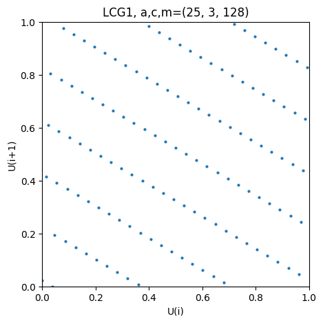
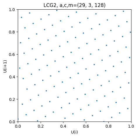
It should be noted that the general structure of the lattice is a consequence of the linear affine iteration of LGSs in general. So the only thing we can ask for is small gaps between the lines. This is a consequence of the linear structure of the iteration and it can be shown that all tuples $\vec{u}_i^k$ lie on, at most,

\sqrt[k]{m\cdot k!}

(16)

parallel hyperplanes. For sole multiplicative LCGs with $c=0$ (Lehmer generators, see Payne et al. (1969)) we can make this more specific using the Theorem of Marsaglia Marsaglia (1968): If we find a sequence $c_i,i=\in \{0,\dots,k-1\}$ of positive integers so that

c_0+c_1a+c_2a^2+\dots+c_{k-1}a^{k-1}\equiv 0\text{ mod }m,

(17)

then all points $\vec{u}_i^k$ will lie on at most

|c_0|+|c_1|+\dots+|c_{k-1}|

(18)

hyperplanes.

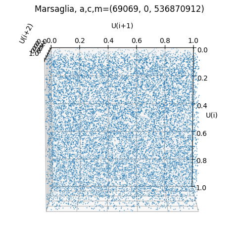
Hereby, he found that the (in)famous RANDU generator with $a=65539, c=0$ and $m=2^29$ has terrible lattice properties. Since

-9+6\cdot 65539-1\cdot 65539^2=4294967296=8\cdot 2^{29}\equiv 0\text{ mod }2^{29},

(19)

all points $\vec{u}_i^3$ lie on at most $|-9|+|6|+|-1|=16$ hyperplanes in 3D. He directly proposed a better one using $a=69069$ instead.

Below we see a visualisation of the 3D-lattice of the two generators.

paramss = {"RANDU": (65539, 0, 2**29), "Marsaglia": (69069, 0, 2**29)}
seed = 1
for name, params in paramss.items():
    lcg = LinearCongruentialGenerator(*params)
    lcg.seed(seed)
    vals = [lcg.draw() for x in range(2**14)] # cannot compute the full period here
    plt.figure(figsize=(6, 6))
    ax = plt.gcf().add_subplot(projection="3d")
    ax.scatter(vals[:-2], vals[1:-1], zs=vals[2:], s=0.2)
    ax.set_xlim([0, 1])
    ax.set_ylim([0, 1])
    ax.set_zlim([0, 1])
    ax.set_xlabel("U(i)")
    ax.set_ylabel("U(i+1)")
    ax.set_zlabel("U(i+2)")
    ax.view_init(elev=100, azim=0, roll=0)
    plt.title(f"{name}, a,c,m={params}")
    plt.show()

    fig = go.Figure(
    data=[
        go.Scatter3d(
            x=vals[:-2],
            y=vals[1:-1],
            z=vals[2:],
            mode='markers',
            marker={'size':1}
            )
        ]
    )
    fig.update_layout(
    scene=dict(
        xaxis_title='U(i)',
        yaxis_title='U(i+1)',
        zaxis_title='U(i+2)'
    ),
    margin=dict(l=0, r=1, b=0, t=1)
    )
    fig.show()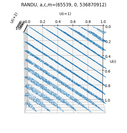

Empirical Tests - Overlapping Permutations Test¶

In contrast to theoretical tests, empirical tests for PRNGs evaluate statistical properties of drawn sequences to see, if they match the behaviour which we would expect if the sequence was indeed IID $U(0,1)$ . The possibilities for defining such tests is almost limitless. We decided to give a simple example in form of the Overlapping Permutations Test.

The idea for this test is comparably simple. Let, as before, $\vec{u}_i^5$ stand for the tuples of five sequential draws $u_i,\dots,u_{i+4}$ and let $\sigma_i$ stand for the sorting permutation of the tuple, then, all $5!=120$ possible permutations should be equally likely. The specific OPERM5 test looks at sequence of one Million random tuples

def overlapping_permutations_test(rng:RNG,n:int=1000000) -> tuple[float,float,dict]:
    """
    Evaluates an Overlapping Permutations Test for a given rng
    with n 5-tuples
    :param rng: random number generator
    :param n: number of tuples to test
    :return: chi2, z_score, and counts or permutations
    """
    perms = list(permutations(range(5))) # all possible permutations
    counts = {p: 0 for  p in perms} # count the occurrences
    for _ in range(n):
        x = [rng.draw() for _ in range(5)] # draw a 5-tuple
        perm = tuple(sorted(range(5), key=lambda i: x[i])) # compute the permutation
        counts[perm]+=1
    expected = n / len(perms)
    chi2 = sum((c - expected) ** 2 / expected for c in counts.values()) # chi^2 test
    df = len(perms)-1
    z_score = (chi2 - df) / math.sqrt(2 * df) # z-score from chi^2 test
    return chi2, z_score,counts

plt.figure(figsize=(10, 5))
indx = 1
for name, params in paramss.items():
    lcg = LinearCongruentialGenerator(*params)
    lcg.seed(seed)
    chi2, z_score,counts = overlapping_permutations_test(lcg,100000)
    perms = list(counts.keys())
    perms.sort()
    cts = [counts[k] for k in perms]
    plt.subplot(2,1,indx)
    indx+=1
    plt.bar(range(len(cts)),cts)
    plt.plot([0,len(cts)-1],[sum(cts)/120,sum(cts)/120],'r') # expected number
    plt.ylabel('samples per permutation-bin')
    plt.title(f"{name}, a,c,m={params}, chi^2={chi2:.03f}, z-score={z_score:.03f}")
plt.show()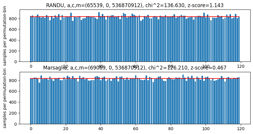

To systematically test PRNGs, there are now entire test suites designed essentially to certify the PRNG. Only if the generator passes every test in the suite is it considered sufficiently secure.

In 1996, Knuth published an initial battery of statistical tests (see, Knuth (1969)), which were later extended to the Diehard by Marsaglia in 1996. These suites served the basis for the development of even larger and more complex test suites. We want to highlight the Test01 with its three sub-suites Small Crush, Crush and Big Crush, last of which consists of 106 different individual empirical tests. The Python-default Mersenne Twister generator passes Diehard and the Small Crush, but fails for several parts of the Crush and Big Crush test. Therefore it is not considered cryptographically safe.

Generation of Arbitrarily Distributed PRNs¶

The usability of a $U(0,1)$ uniformly distributed PRNs $U_i,i\in \{1,\dots,\}$ is surprisingly versatile since they can be transformed to almost any other distribution. The most universal method to do so is the inversion method.

Inversion Method¶

In case a distribition $D$ for a random number $X$ is defined by a known cumulative distribution function $F$ , i.e. $P(X<x)=F(x)$ , then $F(X)\sim U(0,1)$ . The statement follows from the simple transformation

P(F(X)<u)=P(X<F^{-1}(u))=F(F^{-1}(u))=u,

(20)

which implies that the density function of $F(X)$ is the identify on $[0,1)$ , which only the uniform distribution fulfils.

Anyhow, this means, if $U\sim U(0,1)$ , then $F^{-1}(U)\sim D$ . So, any $U(0,1)$ distributed random number $U$ can be transformed into the desired distribution by evaluating $F^{-1}$ on it.

we empirically test it via the exponential distribution with cumulative distribution function $F(x)=1-e^{-\lambda x}$ . Clearly,

F^{-1}(u)=-\frac{1}{\lambda}ln(1-u)

(21)

lam = 1.0
Finv = lambda y: -np.log(1 - y) / lam
rng = LinearCongruentialGenerator(69069, 0, 2**29)
rng.seed(12345)

X = [Finv(rng.draw()) for x in range(10000)]
plt.figure()
plt.hist(X, density=True, bins=100,color='b',label='histogram using Polar Method')
plt.plot([x / 100 for x in range(1000)], [lam * np.exp(-lam * x / 100) for x in range(1000)],color='r',label='analytic density fct')
plt.legend()
plt.show()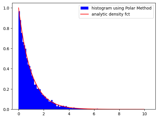

The main problem with the inversion method is that an analytically computable distribution function must be available in order to evaluate it. Whilst this works well for distributions such as the exponential, Weibull or Erlang distributions, the method fails in the case of the normal distribution, amongst others, because

\int_{-\infty}^{x}\frac{1}{\sqrt{2\pi}}e^{-s^2/2}ds

(22)

has not closed analytic form. As a result, some distributions require alternative approaches.

Polar-Method for Normal Distributed PRNs¶

One example for such a method is the Polar-methodMarsaglia & Bray (1964). The concept is to draw tuples $u_1,u_2$ of $U(-1,1)$ IID numbers until

s^2:=u_1^2+u_2^2<1.

(23)

Then, the two numbers

n_1:=u_1\sqrt{\frac{-2\ln(s^2)}{s^2}},\quad n_2:=u_2\sqrt{\frac{-2\ln(s^2)}{s^2}}

(24)

are IID standard normal distributed.

def draw_normal(rng:RNG) -> tuple[float,float]:
    """
    Returns two standard normal distributed PRNs using the Polar Method
    :param rng: instance of a random number generator
    :return: tuple with two IID standard normal distributed PRNs
    """
    while True:
        u1 = 2*rng.draw()-1
        u2 = 2*rng.draw()-1
        s2 = u1**2+u2**2
        if 0<s2<1:
            sq = np.sqrt(-2*np.log(s2)/s2)
            return u1*sq,u2*sq

rng = LinearCongruentialGenerator(69069, 0, 2**29)
rng.seed(12345)
iters = 10000
X = list()
for i in range(iters//2):
    X.extend(draw_normal(rng))
plt.figure()
plt.hist(X, density=True, bins=100,color='b',label='histogram using Polar Method')
xs = np.linspace(-4,4,200)
plt.plot(xs, [1/np.sqrt(np.pi*2)*np.exp(-x**2/2) for x in xs],color='r',label='analytic density fct')
plt.legend()
plt.show()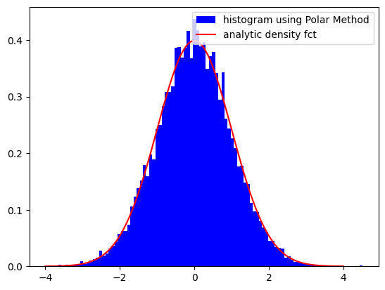

Drawing from Discrete Distributions - Iterative vs. Alias Method¶

Finally, we discuss methods for drawing from discrete distributions. I.e. we want to draw from a random variable $X$ with values in $\{x_1,\dots,x_n\}$ knowing the corresponding vector of probabilities $\vec{p}:=(p_i)_{i=1}^{n}=(P(X=x_i))_{i=1}^{n}$ . It is generally easier to interpret this by as random variable $X'$ on the integer interval $[1,\dots,n]$ , with $P(X'=i)=P(X=x_i)$ .

Iterative Strategy The traditional way to draw from such a vector is conceptually related to the (already discussed) inversion method for $X'$ . We define

F(k):=P(X'\geq k)=\sum_{i=1}^{k}p_i,

(25)

then $F(X')$ is uniformly distributed on $U(0,1)$ . Since $F$ has discrete values, inversion is not directly possible, but can be done using iterations: Draw $u\sim U(0,1)$ and iterate $i$ from 1 to $n$ until $F(i)$ is greater or equal to $u$ and return $i$ (and $x_i$ , respectively).

def draw_discrete(rng:RNG,p:np.ndarray) -> int:
    """
    Draws a random index between 0 and n-1 whereas n is the length of a given probability/weight vector p.
    :param rng: random number generator
    :param p: vector of probabilities, must sum to one!
    :return: random index
    """
    u = rng.draw()
    F = 0
    for i,p in enumerate(p):
        F+=p
        if F>=u:
            return i
    return len(p)-1 #this should not happen if sum(p)==1

x = ['ardberg','ballantines','cragganmore','dalwhinnie']
weights = [5,2,4,1]
p = np.array(weights)/sum(weights)

rng = LinearCongruentialGenerator(69069, 0, 2**29)
rng.seed(12345)
iters = 1000
X = [draw_discrete(rng,p) for i in range(iters)]
plt.figure()
xs = list()
ys_ana = list()
ys_hist = list()
tcks_x = list()
tcks_l = list()
for i,(prob,name) in enumerate(zip(p,x)):
    tcks_x.append(i)
    tcks_l.append(name)
    xs.extend([i-0.5,i+0.5])
    ys_ana.extend([prob,prob])
    v = len([x for x in X if x==i])
    ys_hist.extend([v/iters,v/iters])
plt.fill_between(xs, ys_hist,[0 for y in ys_hist], color='b',label='histogram')
plt.plot(xs, ys_ana,color='r',label='analytic probability fct')
plt.xticks(tcks_x,tcks_l)
plt.legend()
plt.show()

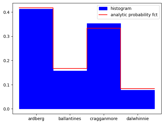
This strategy generally works very well and is easy to implement, but it has one significant weakness: iteration. Essentially, the computational cost increases linearly with the length of the probability vector ( $\mathcal{O}(n)$ ), which means that efficient sampling is no longer so straightforward.

If items need to be retrieved from the list frequently, a pre-processing step can help to reduce the computational efforts. For example, a vector $F$ calculated in advance combined with an efficient search strategy such as bisection can reduce the computational effort to $\mathcal{O}(log(n))$ plus the one-time costs for pre-processing. The Alias method increases efficiency even further.

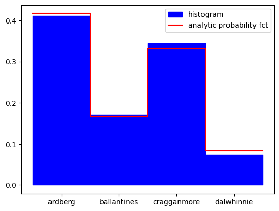
Alias Method The method published first by Alastari Walker Walker (1974) reduces the computational costs for drawing to $\mathcal{O}(1)$ on the costs of a preprocessing step with effort $\mathcal{O}(n\log(n))$ . It is based on the idea displayed in the figure below for the probability vector

\vec{p}=\left(\frac{5}{12},\frac{2}{12},\frac{4}{12},\frac{1}{12}\right)^T.

(26)

The algorithm is best understood interpreting probability as area: Every element $i$ of $\vec{p}$ can be interpreted as the area of a rectangle with sidelengths 1 and $p_i$ . In the preprocessing for the alias method the rectangles are iteratively “squashed” into $n$ rectangles with equal height - and therefore equal probability of $1/n$ . In every iteration, the algorithm first looks for the rectangle with some deficit to the target height $1/n$ . Thereafter, it looks for a rectangle with some overshoot and fills the deficit with it (even if this creates a new deficit). In the first step in the figure below, bin 4 has the largest deficite since $\frac{1}{4}-p_4=\frac{1}{4}-\frac{1}{12}=\frac{2}{12}$ . To fill the bin with the missing we may cut the corresponding part of e.g. bin 1 since it has an overshoot. After this step, bin 4 is full and contains $1/12$ of 4 and $2/12$ of 1. We memorise the ratio $\frac{1/12}{1/4}=\frac{1}{3}$ and which bin was used to fill the gap, i.e. bin 1. These two numbers will be written into the final results of the preprocessing which is a probability table $\vec{U}\in [0,1]^n$ and an alias table $\vec{K}\in \{0,\dots,n\}^n$ .

Since the procedure conserves the area, probability is not lost but only redistributed in a traceable way. We find

p_i=\frac{1}{n}\left(U_i+\sum_{j\in \{1,\dots,n\}:K_j=i}(1-U_j)\right).

(27)

We can exploit this feature by drawing two random numbers: one discrete uniformly distributed number $I$ between 1 and $n$ and one $U(0,1)$ number $U$ . By picking bin $I$ and returninig either $I$ or $K_I$ dependent on whether $U$ is smaller or larger than $U_I$ we draw according to the original probability distriution. This is visually clear, but can also be proven formally:

Defining

X'=\left\lbrace \begin{array}{cc}I& U\leq U_I,\\ K_I&U>U_I\end{array}\right.,

(28)

we get

P(X'=i)=P(I=i)P(U\leq U_i)+\sum_{j\in \{1,\dots,n\}:K_j=i}P(I=j)P(U>U_j)=\frac{1}{n}U_i+\sum_{j\in \{1,\dots,n\}:K_j=i}\frac{1}{n}(1-U_j)=p_i.

(29)

Given the probability and an alias table, the effort required to generate a random variable is reduced to drawing two uniformly distributed random variables, meaning that no iteration is necessary whatsoever. Since the efforts for generating the two tables is considerably larger than the original iterative drawing concept, however, it should be noted that this strategy is only beneficial if a large number of random numbers from the same distribution are required.

def make_tables(p_orig:np.ndarray) -> tuple[list[float],list[int]]:
    """
    Creates a probability and an alias table for the alias algorithm (Walker/Vose)
    :param p_orig: probability vector
    :return: probability and alias table as lists
    """
    n = len(p_orig)
    p = p_orig/sum(p_orig)*n # norm, so that every bin should have value of one
    toosmall = [[i,p] for i,p in enumerate(p) if p<1]
    toolarge = [[i,p] for i,p in enumerate(p) if p>1]
    prob_table = [1.0 for x in range(n)] #default is 1.0
    alias_table = [-1 for x in range(n)] #-1 as default
    while len(toosmall) > 0: # fill the gaps until everything is full
        if len(toolarge)==0: # guard for numerical inaccuracy
            break
        l = toosmall.pop()
        prob_table[l[0]] = l[1]
        g = toolarge.pop()
        alias_table[l[0]] = g[0]
        g[1]-=1-l[1]
        if g[1]<1:
            toosmall.append(g)
        elif g[1]>1:
            toolarge.append(g)
    return prob_table,alias_table

def draw_discrete_alias(rng:RNG,prob_table:list[float],alias_table:list[int]) -> int:
    """
    Discrete draw using the alias algorithm.
    Requires correspondin preprocessing of the probability vector.
    :param rng: random number generator
    :param prob_table: probability table
    :param alias_table: alias table
    :return:
    """
    n = len(prob_table)
    i = int(n*rng.draw())
    if prob_table[i]==1.0: # if prob == 1 we dont need to draw a second rng
        return i
    else:
        u = rng.draw()
        if u<=prob_table[i]:
            return i
        else:
            return alias_table[i]

x = ['ardberg','ballantines','cragganmore','dalwhinnie']
weights = [5,2,4,1]
p = np.array(weights)/sum(weights)

# test if the algorithm works
rng = LinearCongruentialGenerator(69069, 0, 2**29)
rng.seed(12345)
iters = 1000
prob_table, alias_table = make_tables(p)
X = [draw_discrete_alias(rng,prob_table, alias_table) for i in range(iters)]
plt.figure()
xs = list()
ys_ana = list()
ys_hist = list()
tcks_x = list()
tcks_l = list()
for i,(prob,name) in enumerate(zip(p,x)):
    tcks_x.append(i)
    tcks_l.append(name)
    xs.extend([i-0.5,i+0.5])
    ys_ana.extend([prob,prob])
    v = len([x for x in X if x==i])
    ys_hist.extend([v/iters,v/iters])
plt.fill_between(xs, ys_hist,[0 for y in ys_hist], color='b',label='histogram')
plt.plot(xs, ys_ana,color='r',label='analytic probability fct')
plt.xticks(tcks_x,tcks_l)
plt.legend()
plt.show()

# speed benchmarks
p = np.array([rng.draw() for i in range(1000)])
iters = 1000

p /= sum(p)
cl = Clock()
cl.start()
[draw_discrete(rng,p) for x in range(iters)]
cl.stop(f'iterative drawing')
cl.start()
prob_table, alias_table = make_tables(p)
cl.stop(f'alias preprocessing')
cl.start()
[draw_discrete_alias(rng,prob_table, alias_table) for x in range(iters)]
cl.stop(f'alias drawing')

iterative drawing: 0.145147 seconds
alias preprocessing: 0.007407 seconds
alias drawing: 0.002222 seconds

datetime.timedelta(microseconds=2222)

References¶

Von Neumann, J., & others. (1963). Various techniques used in connection with random digits. John von Neumann, Collected Works, 5(768–770), 1.
Thomson, W. E. (1958). A Modified Congruence Method of Generating Pseudo-random Numbers. The Computer Journal, 1(2), 83–83. 10.1093/comjnl/1.2.83
Hull, T. E., & Dobell, A. R. (1962). Random Number Generators. SIAM Review, 4(3), 230–254. 10.1137/1004061
Matsumoto, M., & Nishimura, T. (1998). Mersenne twister: a 623-dimensionally equidistributed uniform pseudo-random number generator. ACM Transactions on Modeling and Computer Simulation, 8(1), 3–30. 10.1145/272991.272995
Payne, W. H., Rabung, J. R., & Bogyo, T. P. (1969). Coding the Lehmer pseudo-random number generator. Communications of the ACM, 12(2), 85–86. 10.1145/362848.362860
Marsaglia, G. (1968). RANDOM NUMBERS FALL MAINLY IN THE PLANES. Proceedings of the National Academy of Sciences, 61(1), 25–28. 10.1073/pnas.61.1.25
Knuth, D. E. (1969). The art of computer. Seminumercial Algorithms, 2, 268–278.
Marsaglia, G., & Bray, T. A. (1964). A Convenient Method for Generating Normal Variables. SIAM Review, 6(3), 260–264. 10.1137/1006063
Walker, A. J. (1974). New fast method for generating discrete random numbers with arbitrary frequency distributions. Electronics Letters, 10(8), 127–128. 10.1049/el:19740097