Case Study: Epi-Vacc - Modelling and Simulation Cookbook

EpiVacc is a multi-method model to simulate the impact of vaccine interventions against endemic diseases. This case study illustrates how the different modelling approaches work together and create an impact.

Topics:

Multi Method Modelling

Objectives:

How to model vaccine interventions and their impact?
What outcomes can be regarded and how can they be put in contrast?
How does hybrid / multi-method modelling enable this?

import io
import json
import os
import shutil
import zipfile

import holoviews as hv
import numpy as np
import requests
from epi_vacc import (
    Config,
    ImmunityModel,
    PrimaryOutcomeId,
    PrimaryOutcomesModel,
    Scenario,
    SecondaryOutcomesModel,
    UncertaintyScenario,
)
from matplotlib import pyplot as plt
from scipy.integrate import solve_ivp

hv.extension("bokeh")

Background¶

Whether a vaccination program is funded by the health care system is an important and complex decision. The costs of purchasing and administering vaccines must be put in contrast with the population’s higher immune competence, the corresponding improved public health, and the related savings from a payer’s perspective due to the reduced burden of the disease. While the decision on whether one vaccination program should be funded by the system is already complex and multifaceted, it becomes particularly challenging when a decision for individual programs must be made at the expense of others due to financial constraints.

In the summer of 2024, the Federal Ministry of Health commissioned the TU Wien to carry out a study Bicher et al. (2025) analysing which vaccination programs would deliver the greatest benefit to the population for the 2025/2026 vaccination season. The aim of this study was to determine how the available budget could best be used to fund vaccinations programs (i.e. by reimbursing vaccination costs). The MoH, supported by their vaccination board (Nationales Impfgremium) proposed 15 different vaccination programs against 9 different pathogens:

Target Pathogen	Who	Scheme
Pertussis	15+ years	5-annual booster
Hepatitis B	15–60 year old who did not receive a vaccination as child	3-stage base immunisation
Pneumococci	60+ and risk persons	Single shot
Meningokocci	Children until 10 + risk persons from 25 (two different vaccines)	4-/3-stage base immunisation & 5-annual booster for risk group
Tick-borne Encephalitis	All	Base immunisation + 5-/3-annual booster
VZV (Varicella)	Children	2-stage base immunisation
VZV (Herpes-Zoster)	60+	2-stage immunisation
Influenza	All / 60+ and risk persons	Seasonal booster
COVID-19	12+ / 60+ and risk persons	Seasonal booster
RSV	Pregnant / infants / 60+	Single shot

At this point, there was little to no evidence on which of them they could afford with the given budget, and which would have the most benefit - and what could be regarded as benefit after all.

PICO Questions¶

In collaboration with the MoH the programs were translated into 70 PICO (Population-Intervention-Comparator-Outcomes) questions (see, Engen et al. (2024)). These questions clearly specified the target population (e.g. children, 60+, risk-persons), the planned intervention (e.g. seasonal booster shot against Influenza), the comparator in the absence of the intervention (no vaccinations, continued status-quo, all vaccinations paid privately) and the investigated outcomes (e.g. vaccination costs, mild/severe/death cases, treatment/hospitalisation costs). For most of the 15 programs, different PICO questions with different assumptions on the adherence of the target population, i.e. how many persons would take the vaccinations, were formulated. For more details, we refer to the published project report Bicher et al. (2025).

Modelling Challenges¶

At first, the problem seems to be a perfect application for epidemiological models, and indeed, the evaluation of vaccinations is one of the core application areas of these models. However, upon closer examination of the task, one finds oneself entering a rabbit hole, confronted with a multitude of challenges that quickly render a perfectly reasonable case study impossible. The most important are likely (see also Bicher et al. (2026)):

Remain unbiased in the light of heterogeneous pathogens and diseases.
Depict the complex nature of real vaccination plans.
Limited availability of data and system knowledge.
Finding a representative evaluation time interval.

As a result, initial attempts to model the system using an agent-based approach, based on the GEPOC ABM population model (see Bicher et al. (2018)) failed. A more simplistic yet more applicable approach was found using a multi-method approach.

Conceptual and Implemented Model¶

The overall model strategy is depicted in Figure 1 and published in Bicher et al. (2026). We will not go into the details of each model here but only point out that the overall model structure consists of Markov-model type immunity model, a SIRVS-type epidemiologcal compartment model, and linear, static Primary and Secondary Outcomes models.

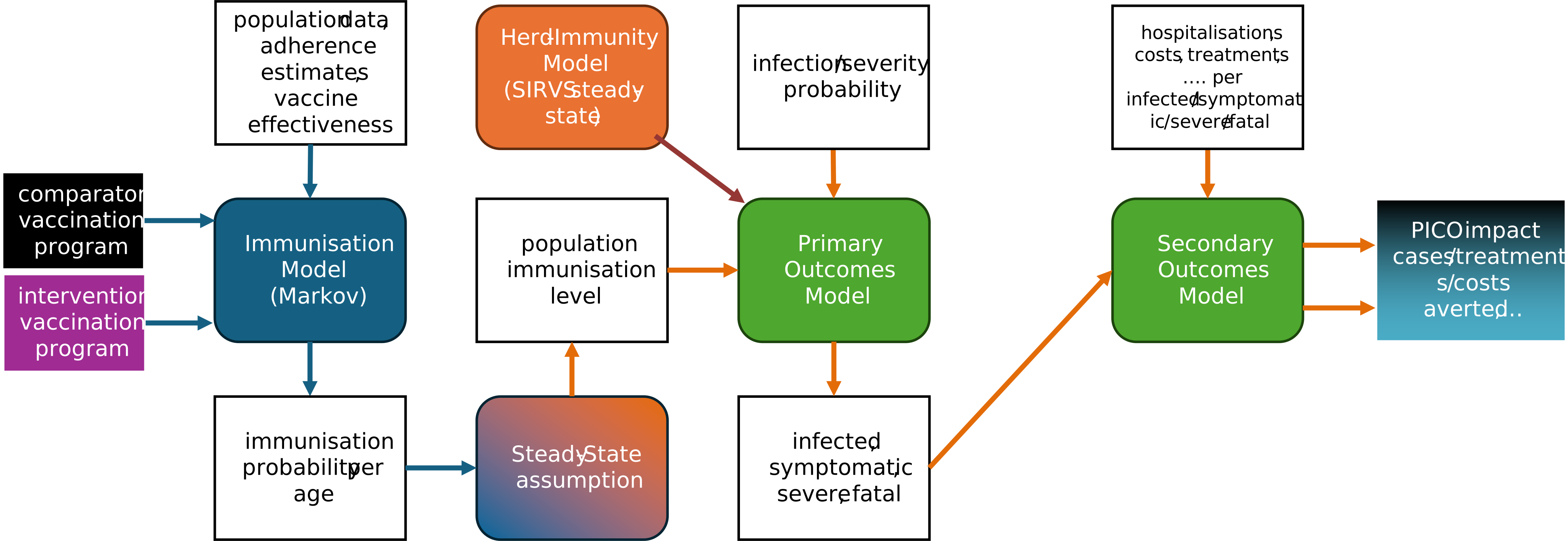
Figure 1:Multi-method concept of the EpiVacc model. Results from an immunity model (Markov-model), and from a SIRVS-type compartment model (differential equation model) feed into a Primary and Secondary Outcomes model (linear, static) to compute the impact of vaccination programs.

The model, henceforth referred to as EpiVacc is implemented in Python3 and found as package epi_vacc publicly in this git repository. We will iteratively explain how the model/package works and is used.

Model Configuration¶

Any experiment with the model requires the setup of a config-file in JSON format. This file contains all information about the PICO question and parameter values. The git repository provides two sample config files, one for a PICO related to Influenza vaccinations, one related to Hepatitis-B. We have a quick look into them.

url = "https://gitlab.tuwien.ac.at/martin.bicher/vacc_eval/-/archive/1.0.1/vacc_eval-1.0.1.zip"

# Download the zip file into memory
response = requests.get(url)
response.raise_for_status()

# the package requires a lot of things to be saved locally for reproducibility reasons
# so we need to make a temporary folder here
localfolder = "./temp/"
if not os.path.isdir(localfolder):
    os.mkdir(localfolder)

# Load zip from memory and download the config files locally
with zipfile.ZipFile(io.BytesIO(response.content)) as z:
    ids = ["INF", "HEP"]  # ids for influenza and hepatitis
    configs = dict()
    for id in ids:
        fn = id + ".json"
        with z.open("vacc_eval-1.0.1/configs/" + fn, "r") as f:
            json_format = json.load(f)  # load the file in JSON format
        json_format["resultFolder"] = (
            localfolder
            # change the folder where the simulation should save the results
        )
        with open(localfolder + fn, "w") as f:
            print(os.path.abspath(f.name))
            json.dump(json_format, f)  # dump locally
        config = Config(localfolder + fn)  # finally, open it as a config-object
        configs[id] = config

print("print some fields to get an idea on what is included in the JSON file:")
print(configs["INF"].file_content.keys())
print(configs["INF"].file_content["vaccinationStages"])

Model Input: Vaccination Program¶

Mathematically, we define a vaccination program is interpreted as a list $v_j,j\in \{1,\dots,M\}$ of tuples

v_j:=(t_j,r_j,e_j,c_j),

(1)

whereas each tuple characterises one stage of the program. Hereby,

$t_j\in \mathbb{R}^+_0$ stands for the recommended administration age of the vaccination shot
$r_j\in [0,1]$ refers to the expected participation among the population with age $t_j$
$e_j\in [0,1]$ refers to the effectiveness of the vaccine against a certain outcome, i.e. how well the vaccine protects the individual, and
$c_j \in \mathbb{R}^+_0$ stands for the costs associated with administering the vaccination stage.

In full detail, $r_j$ is sub-population dependent (e.g. risk population, pregrant,...), $e_j$ depends on the outcome of interest (e.g. infection, symptomatic, severe, ...), and $c_j$ depends on the payer or payment program (e.g. privately paid, child-vaccination budget, ...).

Below we illustrate the comparator and intervention program against Hepatitis-B. The program is depicted with three sub-populations: base12 refers to the part of the population who get the first dose as a child with the age of 0 and the booster shot with 7. Those in base1 had the first one, but missed out the booster shot. The other show vaccination stages depict a refreshment vaccinations for those which could or did not want to participante in the (full) base immunisation program. To depict that the refreshment can be taken any time between age 16 and 60, multiple vaccination events with reduced participation are depicted. In the comparator, which should depict the status-quo, the refreshment is only taken by the base1 sub-population and is currently paid privatey, in the intervention, also the others subpopulation may get the vaccine and it is reimbursed.

def visualise_vacc_program(config: Config, scenario: Scenario) -> None:
    """
    Visualises the different stages of the configured vaccination program
    :param config: instance of the Config class
    :param scenario: one of Scenario.FIT,Scenario.COMPARATOR or Scenario.INTERVENTION
    """
    pops = config.sub_populations
    cmp = plt.get_cmap("viridis")
    k = 0
    for i, (p, r) in enumerate(pops.items()):
        plt.fill_between(
            [0, 100],
            [k, k],
            [k + r, k + r],
            color=cmp(i / len(pops.keys())),
            alpha=0.2,
            label=p,
        )
        k += r
    for stage in config.vaccination_stages[scenario]:
        a = stage.get_age()
        k = 0
        for p, r in pops.items():
            plt.plot(
                [a, a],
                [k, k + stage.get_participant_ratio(p) * r],
                color="r",
                linewidth=3,
            )
            k += r
    plt.legend()


plt.figure(figsize=(8, 6))
plt.subplot(2, 1, 1)
visualise_vacc_program(configs["HEP"], Scenario.COMPARATOR)
plt.title("Hepatitis-B, Comparator")
plt.xlim([0, 100])
plt.ylim([0, 1])
plt.subplot(2, 1, 2)
visualise_vacc_program(configs["HEP"], Scenario.INTERVENTION)
plt.title("Hepatitis-B, Intervention")
plt.xlim([0, 100])
plt.ylim([0, 1])
plt.tight_layout()
plt.show()

Immunity Model¶

For every individual, we define a stochastic process $X(t)$ modeling whether an individual is (1) or is not (0) protected against a certain outcome at precise age $t$ due to a vaccination. We furthermore aim to model

\mu:\mathbb{R}^+\rightarrow [0,1]:t\mapsto \mu(t):=P(X(t)=1),

(2)

henceforth called vaccine-induced-immunity curve.

In the model we assume that $X$ is a Markov process: Transition $1\rightarrow 0$ reflects waning of immunity. For our model, we assume that this process is memoryless (Markov process) with rate $\alpha$ , meaning that the immunity waning times are exponentially distributed. As a result, for any two $t_2>t_1$

\mu(t_2)=P(X(t_2)=1) = P(X(t_2)=1|X(t_1)=1)P(X(t_1)=1)=\exp(-\alpha(t_2-t_1))\mu(t_1).

(3)

Transition $0\rightarrow 1$ is externally triggered by the vaccination stages. For the $j$ -th stage at age $t_j$ we find, that the person has a likelihood of $r_j$ to participate in the program, and a likelihood of $e_j$ to gain immunity from the vaccination stage.

Let $X_j^-:=\lim_{t\rightarrow t_j^-}X(t)$ define the state of the process right before the vaccination and $\mu^{-}_j:=P(X_j^-=1)$ , then

\mu(t_j)=P(X(t_j)=1)=P(X(t_j)=1|X_j^-=1)\mu^{-}_j+P(X(t_j)=1|X_j^-=0)(1-\mu^{-}_j) = \mu^{-}_j+r_je_j(1-\mu^{-}_j).

(4)

Combining the two equations provides $\mu$ for arbitrary points in time.

We compute some immunity curves for different outcomes below. For Hepatitis-B we asumed no difference in protectivity against different outcomes, for Influena, however, data shows a declining protection against symptomatic disease for the elderly. In general protection levels against Influena can be seen on a much lower level due to (a) much faster waning, (b) smaller participant ratios, and (c) lower estimates for vaccine effectiveness.

cmp = plt.get_cmap("viridis")
IMMUNITY_RESULTS = dict()
for id in ["HEP", "INF"]:
    IMMUNITY_RESULTS[id] = dict()
    # first, compute all immunity results and save them for later
    for sc in [Scenario.FIT, Scenario.COMPARATOR, Scenario.INTERVENTION]:
        for usc in [
            UncertaintyScenario.MAIN,
            UncertaintyScenario.LOW,
            UncertaintyScenario.HIGH,
        ]:
            IMMUNITY_RESULTS[id][(sc, usc)] = dict()
            for po in [
                PrimaryOutcomeId.INFECTED,
                PrimaryOutcomeId.SYMPTOMATIC,
                PrimaryOutcomeId.SEVERE,
                PrimaryOutcomeId.FATAL,
            ]:
                if (
                    po is PrimaryOutcomeId.INFECTED
                    and not configs[id].compute_herd_effect
                ):
                    IMMUNITY_RESULTS[id][(sc, usc)][po] = (None, None)
                else:
                    imdl = ImmunityModel(configs[id], po, sc, usc)
                    res, res_supop = imdl.run()
                    IMMUNITY_RESULTS[id][(sc, usc)][po] = (
                        res.get_average_immunity_vector(),
                        res,
                    )
    # now, plot some of them
    plts = list()
    for i, po in enumerate(
        [
            PrimaryOutcomeId.INFECTED,
            PrimaryOutcomeId.SYMPTOMATIC,
            PrimaryOutcomeId.SEVERE,
            PrimaryOutcomeId.FATAL,
        ]
    ):
        res = IMMUNITY_RESULTS[id][(Scenario.INTERVENTION, UncertaintyScenario.MAIN)][
            po
        ]
        if res[0] is None:  # no herd immunity effects
            continue
        T = np.linspace(0, 100, 1000)
        X = [res[1].get_immunity(t) for t in T]
        plts.append(hv.Curve((T, X), label=po.name.lower()).opts(color=cmp(i / 3)))
    plot = hv.Overlay(plts).opts(
        show_legend=True,
        legend_position="top_right",
        xlabel="age",
        ylabel="immunity probability",
        xlim=(0, 100),
        ylim=(0, 1),
        title="immunity against " + id,
        responsive=True,
        height=400,
        max_width=1000,
    )
    display(plot)

Steady-State Property¶

To quantify the impact of the immunity level on the disease outcomes, we apply a steady-state assumption. I.e. we assume, that the population size (per age= remains constant and that the vaccination program (comparator or intervention) is sufficiently long in place to cause the same level of annual infections/cases and the same level of immunity. As a result, the average likelihood that a person between age $a$ and $a+1$ is immunised is representative for the immunisation likeliood of the whole age cohort $a$ :

\forall a\in \{0,1,\dots\}: \mathcal{I}_{a}:=\int_{a}^{a+1}\mu(t)dt,

(5)

and for the overall population by

\mathcal{I}^{tot}:=\frac{\vec{N}\cdot (\mathcal{I})_{a=0}^{100}}{\lVert\vec{N}\rVert_1},

(6)

whereas $\vec{N}=(N_a)_{a=0}^{N}$ stands for size of the age cohorts.

We approximate a yearly cases $O_a$ for a certain age $a$ as

O_a=(1-\mathcal{I}_{a})O_a^0,

(7)

whereas $O_a^0$ stands for the yearly incidence in a naive population without vaccination - which need to be found in a calibration process.

Unfortunately, this solely linear approach neglects nonlinear herd-immunity effects in case the vaccine protects agains infection and transmission (which is not always given). Thus, we slightly extend this formula to

O_a=(1-\mathcal{I}_{a})\Xi(\cdot)O_a^0,

(8)

SIRVS-Model¶

The SIRVS-model (susceptible-infectious-recovered-vaccinated-susceptible) is a well known epidemic compartmental model based on the famous SIR-model by Kermack and McKendrick and unites the SIRS model with the SIRV model. It can be regarded at the simplest model considering herd-immunity effects, immunity-waning, and vaccinations at the same time and is defined by the following system of four coupled differential equations:

\begin{array}{cccccc} \dot{S}(t)&=&-\beta S(t)I(t)&&+\delta_1R(t)+\delta_2V(t)&-\kappa S(t)\\ \dot{I}(t)&=&\beta S(t)I(t)&-\gamma I(t)&&\\ \dot{R}(t)&=&&\gamma I(t)&-\delta_1 R(t)&\\ \dot{V}(t)&=&&&-\delta_2 V(t)&+\kappa S(t)\\ \end{array}

(9)

Although the model dynamics are too complicated to be solved analytically, its steady-state is. By $\dot{S}=\dot{I}=\dot{R}=\dot{V}=0$ we find, for example,

n(\infty)=n_0(\infty)\left(1-\frac{R_0}{R_0-1}V(\infty)\right),

(10)

whereas $n(\infty)$ and $V(\infty)$ stand for the new infections $n(t)=\beta S(t)I(t)$ and total vaccination in the steady state, $n_0$ for the new infections in a system without vaccinations (i.e. $\kappa=0$ ), and $R_0$ for the base reproduction rate $R_0=\frac{\beta}{\gamma}$ of the disease. By splitting the rate into self- and third-party protection, we identify our nonlinearity factor $F$ by

n(\infty)=n_0(\infty)(1-V(\infty))\underbrace{\frac{1-BV(\infty)}{1-V(\infty)}}_{F}

(11)

which, transferred to our age-dependent framework, leads to

\Xi(R_0,\mathcal{I}^{tot})=\frac{1-\frac{R_0}{R_0-1}\mathcal{I}^{tot}}{1-\mathcal{I}^{tot}}.

(12)

We illustrate this factor with the SIRVS model below. It corresponds to the ratio between the two red lines in their steady state (i.e. to the right of the picture).

import json


class SIRVSModel:
    def __init__(
        self, beta: float, gamma: float, delta1: float, delta2: float, kappa: float
    ):
        """
        Implementation of the SIRVS model
        :param beta: infection rate
        :param gamma: recovery rate
        :param delta1: waning rate for recovered
        :param delta2: waning rate for vaccinated
        :param kappa: vaccination rate
        """
        self.beta = beta
        self.gamma = gamma
        self.delta1 = delta1
        self.delta2 = delta2
        self.kappa = kappa

    def rhs(self, t: float, x: np.ndarray) -> np.ndarray:
        """
        Right hand side of the SIRVS differential equation
        :param t: time
        :param x: state vector
        :returns: derivative
        """
        y = np.zeros(4)
        infs = self.beta * x[0] * x[1]
        recs = self.gamma * x[1]
        wanes1 = self.delta1 * x[2]
        wanes2 = self.delta2 * x[3]
        vaccs = self.kappa * x[0]
        y[0] = -infs - vaccs + wanes1 + wanes2
        y[1] = infs - recs
        y[2] = recs - wanes1
        y[3] = vaccs - wanes2
        return y

    def run(self, x0: np.ndarray, tend: float) -> tuple[np.ndarray, np.ndarray]:
        """
        Solves the ode using a runge-kutta solver and returns the results of the model
        :param x0: initial value
        :param tend: simulation end-time
        :returns: vector of time instants and corresponding vector of states
        """
        res = solve_ivp(self.rhs, [0, tend], x0, max_step=1)
        return res.t, res.y


r_0 = 3.0
kappa = 0.003
gamma = 0.2
delta1 = 0.01
delta2 = 0.01
x0 = np.array([0.95, 0.05, 0.0, 0.0])


def sir_plot(r_0: float = 3.0, kappa: float = 0.003) -> hv.Overlay:
    """
    Plots the impact of a certain vaccination rate kappa onto the infection count for
    different values of R_0
    :param r_0: R_0 of the disease
    :param kappa: vaccination rate
    :returns: holoview plot
    """
    beta = r_0 * gamma  # derived from r_0 and recovery time

    tend = 1000  # should be enough for a proper "steady state"

    mdl_novacc = SIRVSModel(
        beta, gamma, delta1, delta2, 0.0
    )  # model without vaccinations
    tt_novacc, xx_novacc = mdl_novacc.run(x0, tend)
    mdl_vacc = SIRVSModel(beta, gamma, delta1, delta2, kappa)  # model with vaccinations
    tt_vacc, xx_vacc = mdl_vacc.run(x0, tend)

    novacc_i = hv.Curve(
        (tt_novacc, xx_novacc[1, :]), label="infected (without vaccinations)"
    ).opts(color=(1.0, 0.0, 0.0))
    vacc_i = hv.Curve(
        (tt_vacc, xx_vacc[1, :]), label="infected (with vaccinations)"
    ).opts(color=(0.7, 0.0, 0.0))
    vacc_v = hv.Curve((tt_vacc, xx_vacc[3, :]), label="vaccinated immune").opts(
        color=(0, 0, 0)
    )
    return (novacc_i * vacc_i * vacc_v).opts(
        xlabel="time",
        ylabel="ratio of the population",
        xlim=(0, tend),
        show_legend=True,
        legend_position="top_right",
        responsive=True,
        height=400,
        max_width=1000,
    )


plot = sir_plot(r_0, kappa)
display(plot)

Outcomes Model and Model Fit¶

With $\mathcal{I}^k_a$ being the immunity against a certain outcome $k$ , e.g. symptomatic or severe disease, and $\mathcal{I}^i_a$ being the immunity against infection, we compute

O_a^i=(1-\mathcal{I}^i_{a})\Xi(\mathcal{I}^{tot,i},R_0)O_a^{0,i},

(13)

whereas $O_a^i,O_a^{0,i}$ refer to the total infections with and without vaccinations and

O_a^k=(1-(\mathcal{I}^k_a-\mathcal{I}^i_a))\Psi_a^kO_a^{i},

(14)

whereas $O_a^k$ stands for the observed cases with outcome $k$ . Factor $\Psi_a^k$ is the age-dependent likelihood that an unvaccinated person of a certain age will develop the more severe outcome $k$ .

Given a certain status-quo vaccination program (in addition to the comparatpor and intervention) we may calibrate the missing factors to given surveillance data for the corresponding diseases (see Figure 2). To be precise, we fit the values of the products $\Psi_a^k\Theta_a$ , whereas $\Theta_a:=\frac{O_a^{0,i}}{P_a}$ is the per-person likelihood for getting infected in the course of a year in the absence of vaccinations. Hence, the fitted product $\Psi_a^k\Theta_a$ can be interpreted as the overall yearly per-person probability for for getting outcome $k$ in the absence of vaccinations.

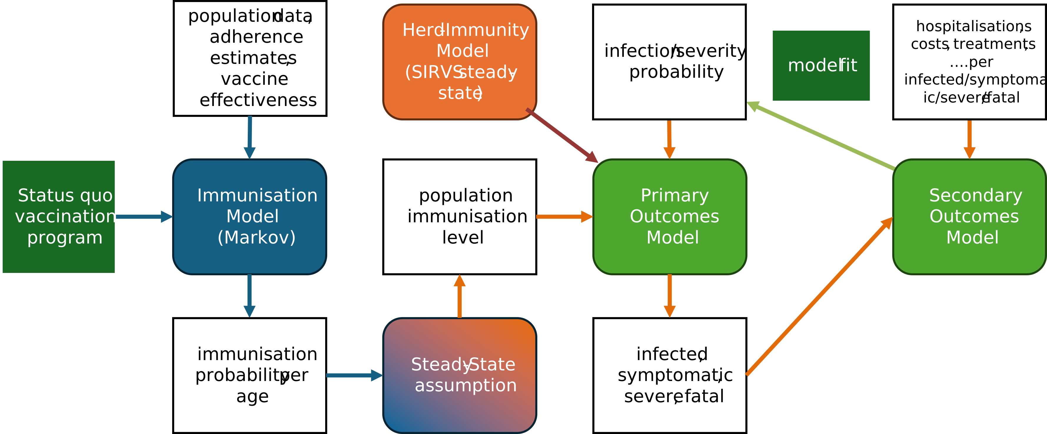
Figure 2:Strategy to fit the model with a status-quo vaccination program and data on certain reference outcomes.

Below we fit the outcomes model given a set of immunity models and show the fitted probabilities $\Psi_a^k\Theta_a$ . While they are somewhat in the same range for Hepatitis-B, they differ heavily for Influenza. For the latter, the likelihood for symptomatic disease is much higher than for more severe outcomes.

cmp = plt.get_cmap("viridis")
FITTED_PARAMS = dict()
sc = Scenario.FIT
usc = UncertaintyScenario.MAIN
for id in ["HEP", "INF"]:
    FITTED_PARAMS[id] = dict()
    plots = list()
    iv_inf = IMMUNITY_RESULTS[id][(sc, usc)][PrimaryOutcomeId.INFECTED][0]
    for i, po in enumerate(
        [PrimaryOutcomeId.SYMPTOMATIC, PrimaryOutcomeId.SEVERE, PrimaryOutcomeId.FATAL]
    ):
        iv_po = IMMUNITY_RESULTS[id][(sc, usc)][po][0]
        pom = PrimaryOutcomesModel(
            configs[id].population, iv_po, iv_inf, configs[id].R0
        )
        ref = configs[id].reference_outcomes_specs[po]
        reference_values = ref.reference_values
        param = pom.fit_to_reference(
            ref.reference_values, ref.kernels_po[po]
        )  # fits the model to the reference data
        FITTED_PARAMS[id][po] = param  # fitted parameters
        plots.append(
            hv.Curve(param.get_age_timeline(), label=po.name.lower()).opts(
                color=cmp(i / 2)
            )
        )
    plot = hv.Overlay(plots).opts(
        xlabel="age",
        ylabel="probability for outcome",
        responsive=True,
        height=400,
        max_width=800,
        title=id,
    )
    display(plot)

Primary Outcomes¶

With the fitted parameters, we can compute the primary outcomes for different immunisation profiles, i.e. the comparator and intervention vaccination plans. We may incorporate parameter uncertainty w.r. to vaccine effectiveness. Since the regarded vaccination plans only differ a little, the differences of the absolute outcomes are very subtle. Nevertheless, the benfit of the intervention is clearly visible.

def plot_comparison_with_uncertainty(
    result_dict: dict[tuple[Scenario, UncertaintyScenario], dict],
    outcomes_key: PrimaryOutcomeId | str,
    title: str,
    ylabel: str = "cases",
) -> hv.Overlay:
    """
    Plots comparator and intervention results with uncertainty interval
    :param result_dict: dictionary object with keys (Scenario,UncertaintyScenario) and
    values as dictionaries mapping outcomes_keys to result
    :param outcomes_key: outcome key to consider, can be string or PrimaryOutcomeId enum
    dependent on the result_dict object
    :param title: title for the plot
    :returns: holoviews plot showing median values and shaded confidence regions for
    comparator and intervention
    """
    median_comp = result_dict[(Scenario.COMPARATOR, UncertaintyScenario.MAIN)][
        outcomes_key
    ].get_age_timeline()
    low_comp = result_dict[(Scenario.COMPARATOR, UncertaintyScenario.LOW)][
        outcomes_key
    ].get_age_timeline()
    high_comp = result_dict[(Scenario.COMPARATOR, UncertaintyScenario.HIGH)][
        outcomes_key
    ].get_age_timeline()
    median_int = result_dict[(Scenario.INTERVENTION, UncertaintyScenario.MAIN)][
        outcomes_key
    ].get_age_timeline()
    low_int = result_dict[(Scenario.INTERVENTION, UncertaintyScenario.LOW)][
        outcomes_key
    ].get_age_timeline()
    high_int = result_dict[(Scenario.INTERVENTION, UncertaintyScenario.HIGH)][
        outcomes_key
    ].get_age_timeline()
    median_diff = (
        result_dict[(Scenario.INTERVENTION, UncertaintyScenario.MAIN)][outcomes_key]
        - result_dict[(Scenario.COMPARATOR, UncertaintyScenario.MAIN)][outcomes_key]
    ).get_age_timeline()
    low_diff = (
        result_dict[(Scenario.INTERVENTION, UncertaintyScenario.LOW)][outcomes_key]
        - result_dict[(Scenario.COMPARATOR, UncertaintyScenario.LOW)][outcomes_key]
    ).get_age_timeline()
    high_diff = (
        result_dict[(Scenario.INTERVENTION, UncertaintyScenario.HIGH)][outcomes_key]
        - result_dict[(Scenario.COMPARATOR, UncertaintyScenario.HIGH)][outcomes_key]
    ).get_age_timeline()

    median_comp_plot = hv.Curve(median_comp, label="comparator (median)").opts(
        color="red"
    )
    ci_comp_plot = hv.Area(
        (median_comp[0], high_comp[1], low_comp[1]),
        label="comparator (90% CI)",
        vdims=["lower", "upper"],
    ).opts(color="red", alpha=0.3)
    median_int_plot = hv.Curve(median_int, label="intervention (median)").opts(
        color="blue"
    )
    ci_int_plot = hv.Area(
        (median_int[0], high_int[1], low_int[1]),
        label="intervention (90% CI)",
        vdims=["lower", "upper"],
    ).opts(color="blue", alpha=0.3)
    comp_plot = (ci_comp_plot * ci_int_plot * median_comp_plot * median_int_plot).opts(
        title=title, xlabel="age", ylabel=ylabel, responsive=True, height=300
    )
    median_diff_plot = hv.Curve(median_diff, label="difference (median)").opts(
        color="black"
    )
    ttl = f"Difference: {sum(median_diff[1]):.01f} ({sum(high_diff[1]):.01f}"
    ttl += f",{sum(low_diff[1]):.01f}) {ylabel}"
    ci_diff_plot = hv.Area(
        (median_diff[0], high_diff[1], low_diff[1]),
        label="difference (90% CI)",
        vdims=["lower", "upper"],
    ).opts(color="black", alpha=0.3)
    diff_plot = (ci_diff_plot * median_diff_plot).opts(
        xlabel="age",
        ylabel=ylabel,
        title=ttl,
        responsive=True,
        height=300,
    )
    return (comp_plot + diff_plot).opts(shared_axes=False)


PRIMARY_OUTCOMES = dict()
for id in ["HEP", "INF"]:
    # compute the results first
    PRIMARY_OUTCOMES[id] = dict()
    for sc in [Scenario.COMPARATOR, Scenario.INTERVENTION]:
        for usc in [
            UncertaintyScenario.LOW,
            UncertaintyScenario.MAIN,
            UncertaintyScenario.HIGH,
        ]:
            key = (sc, usc)
            PRIMARY_OUTCOMES[id][key] = dict()
            for po in [
                PrimaryOutcomeId.SYMPTOMATIC,
                PrimaryOutcomeId.SEVERE,
                PrimaryOutcomeId.FATAL,
            ]:
                iv_inf = IMMUNITY_RESULTS[id][key][PrimaryOutcomeId.INFECTED][0]
                iv_po = IMMUNITY_RESULTS[id][key][po][0]
                pom = PrimaryOutcomesModel(
                    configs[id].population, iv_po, iv_inf, configs[id].R0
                )
                PRIMARY_OUTCOMES[id][key][po] = pom.run(FITTED_PARAMS[id][po])
    # now plot some of the results
    for po in [
        PrimaryOutcomeId.SYMPTOMATIC,
        PrimaryOutcomeId.SEVERE,
        PrimaryOutcomeId.FATAL,
    ]:
        display(
            plot_comparison_with_uncertainty(
                PRIMARY_OUTCOMES[id], po, id + ", " + po.name.capitalize()
            )
        )

Secondary Outcomes¶

Finally, we fully exploit the fitted model. We assume, that any outcome of interest $Q^m$ can be computed as a linear-combination of the primary outcomes, i.e. infected, symptomatic, severe and fatal cases, i.e.

Q^m=\sum_{k}T^{m,k}O^k

(15)

for some kernel matrices $T^k$ . This specification offers lots of freedom for defining outcomes: A zero-matrix will make the result independent of the corresponding primary. A diagonal matrix will create a proportional age-dependent relation, e.g., well suited to model age-dependent treatment costs. Finally, using a triangular matrix makes it possible to model a time-delay between primary and secondary outcome. This is nicely visible for Hepatitis-B (see plots below) for which hospitalized and severe (or milds) have clearly different age distribution.

Comparing these outcomes for the comparator and the intervention program gives estimates for the benefits. However, one should not forget that different interventions are associated with different costs. So it is important to also contrast the benefits with the costs.

SECONDARY_OUTCOMES = dict()
for id in ["HEP", "INF"]:
    msg = f"available secondary outcome specifications for {id}:"
    msg += f"{', '.join(configs[id].secondary_outcomes_specs.keys())}"
    print(msg)
    SECONDARY_OUTCOMES[id] = dict()
    # compute some outcomes first
    for sc in [Scenario.COMPARATOR, Scenario.INTERVENTION]:
        for usc in [
            UncertaintyScenario.LOW,
            UncertaintyScenario.MAIN,
            UncertaintyScenario.HIGH,
        ]:
            key = (sc, usc)
            SECONDARY_OUTCOMES[id][key] = dict()
            for so in [
                "hospitalized",
                "hospitalDays",
                "milds",
                "workingSymptomatic",
                "sickLeaveDays",
            ]:
                secondary_outcome_spec = configs[id].secondary_outcomes_specs[so]
                som = SecondaryOutcomesModel(
                    secondary_outcome_spec.kernels_po, secondary_outcome_spec.kernels_so
                )
                SECONDARY_OUTCOMES[id][key][so] = som.run(
                    PRIMARY_OUTCOMES[id][key], SECONDARY_OUTCOMES[id][key]
                )
    # now plot some results
    display(
        plot_comparison_with_uncertainty(
            PRIMARY_OUTCOMES[id], PrimaryOutcomeId.SEVERE, id + ", severe"
        )
    )
    display(
        plot_comparison_with_uncertainty(
            SECONDARY_OUTCOMES[id],
            "hospitalized",
            id + ", hospitalized",
            "hospitalizations",
        )
    )
    display(
        plot_comparison_with_uncertainty(
            SECONDARY_OUTCOMES[id], "hospitalDays", id + ", hospital days", "days"
        )
    )
    display(
        plot_comparison_with_uncertainty(
            PRIMARY_OUTCOMES[id], PrimaryOutcomeId.SYMPTOMATIC, id + ", symptomatic"
        )
    )
    display(
        plot_comparison_with_uncertainty(
            SECONDARY_OUTCOMES[id],
            "milds",
            id + ", mild cases",
            "extramural treatments",
        )
    )
    display(
        plot_comparison_with_uncertainty(
            SECONDARY_OUTCOMES[id], "sickLeaveDays", id + ", sick leave days", "days"
        )
    )

# close the logger instances
for c in configs.values():
    file_handler = c.logger.handlers[0]
    file_handler.close()
    c.logger.removeHandler(file_handler)
# clean up
try:
    shutil.rmtree(localfolder)
    print("successfully cleaned up")
except OSError:
    print("cleaning up was unsuccessful")

References¶

Bicher, M., Brodersen, J., Erber, A., Geier, P., Jeleff, M., Popper, N., Rippinger, C., Urach, C., Zauner, G., Zechmeister, M., & Zimmermann, C. (2025). Impactevaluierung von Priorisierten Impfungen. TU Wien. 10.48436/sqvcq-qwg65
van Engen, A., Krüger, R., Parnaby, A., Rotaru, M., Ryan, J., Samaha, D., & Tzelis, D. (2024). The impact of additive population (s), intervention, comparator (s), and outcomes in a European joint clinical health technology assessment. Value in Health, 27(12), 1722–1731. 10.1016/j.jval.2024.07.024
Bicher, M., Rippinger, C., Urach, C., Zauner, G., Zechmeister, M., & Niki, P. (2026, June). Mathematical Modeling Framework for Comparison of Vaccination Strategies for Different Diseases. Proceedings of the 40th ACM SIGSIM Conference on Principles of Advanced Discrete Simulation.
Bicher, M., Urach, C., & Popper, N. (2018). Gepoc ABM: a generic agent-based population model for Austria. 2018 Winter Simulation Conference (WSC), 2656–2667. 10.1109/WSC.2018.8632170
Bicher, M., Rippinger, C., Urach, C., Zauner, G., Zechmeister, M., & Popper, N. (2026). Mathematical Modeling Framework for Comparison of Vaccination Strategies for Different Diseases. Proceedings of the 40th ACM SIGSIM International Conference on Principles of Advanced Discrete Simulation, 116–126. 10.48436/sqvcq-qwg65