Case Study: Epidemic Model - Modelling and Simulation Cookbook

We model the spread of an epidemic using a cellular automaton.

Topics:

Cellular Automata

Objectives:

Understand the core mechanics of a cellular automaton and how they can be used to model complex real-world phenomena.
How does the practical implementation of a cellular automaton work from scratch?
How does our parameter selection influence the outcome of the simulation?

import numpy as np
import copy
from matplotlib import pyplot as plt
from matplotlib import colors as mcolors
from matplotlib import animation, patches
from IPython.display import HTML

Motivation / System¶

We want to model the spread of disease through a population and track the number of infected, recovered and susceptible people. Our goal is to understand the impact of local effects on vaccinations. Since traditional compartmental models (differential equation / System Dynamics) cannot depict local effects we choose a strategy based on cellular automata.

Conceptual Model¶

The model is based on the approach presented in Bicher & Popper (2013), however multiple very similar models can be found throughout the international literature.

Cells and Cell Arrangement¶

We opt for a grid with $M\times N$ rectangularly aligned cells. I.e. every cell is addressed by the tuple $(i,j),i\in \{1,\dots,M\},j\in \{1,\dots,N\}$ .

States and State-Space¶

Each cell can have four possible states:

susceptible $S$
infectious $I$
recovered $R$
vaccinated $V$

Neighbourhood¶

The specific neighbourhood will be one of the key parameters of the model. In the figure below we see a graphical representation of the different supported neighbourhood types. The neighbourhood is cropped at the borders.

Update Rule¶

The following state-changes are possible:

$S\rightarrow I$ , susceptible to infectious, depends on the states of the neighbours. In case one or more neighbours are in the $I$ state, the cell can change its state to infected with a certain probability $p_i$ .
$S\rightarrow V$ , susceptible to vaccinated, will be triggered with probability $p_v$ , regardeless of the neighbours. If, by chance, the cell were to become infected and vaccinated at the same time, we will consider the vaccination to have failed and the cell will become infected.
$I\rightarrow R/S$ , infectious to recovered/susceptible, will be triggered with probability $p_r$ . That means, on average, a cell will remain infectious for $1/p_r$ timesteps. If the recovered cell switches to the $R$ state (SIR type model) or the $S$ state (SIS type model) will be left open for parametrisation (model-type).

In all other cases, the states of the cell does not change.

Implemented Model¶

Below, we define a class to handle our model. When creating an instance of the EpisimCA class we can adjust the model with the model_type parameter.

class EpisimCA:
    """
    A class handling the model logic of our cellular automaton.
    """
    def __init__(self,
                 model_type: str = "SIR",
                 grid_dimensions: tuple = (50, 50),
                 infection_probability: float = 0.4,
                 recovery_probability: float = 0.2,
                 vaccination_probability: float = 0.0,
                 start_frac_infected: float = 0.01,
                 start_num_infected: int = None,
                 start_frac_vaccinated: float = 0.0,
                 start_num_vaccinated: int = None,
                 seed : int = 12345) -> None:
        """
        Creates a new SIR/SIS type cellular automata model
        :param model_type: Whether to use the SIR or SIS model. Default is "SIR".
        :param grid_dimensions: Dimensions of the grid. Default is (50, 50).
        :param infection_probability: Probability of a susceptible cell to be infected.
        :param recovery_probability: Probability of an infected cell to become recovered.
        :param start_frac_infected: Fraction of cells to be infected at the start of the simulation.
        :param start_num_infected:  Number of infected cells at the start of the simulation. If set this will overwrite the start_frac_infected parameter.
        :param start_frac_vaccinated: Fraction of cells to be vaccinated at the start of the simulation.
        :param start_num_vaccinated: Number of vaccinated cells at the start of the simulation. If set this will overwrite the start_frac_vaccinated parameter.
        :param seed: seed for the random number generator to make experiments reproducible
        """

        self.rng = np.random.default_rng(seed=seed)
        self.model_type = model_type
        self.infection_probability = infection_probability
        self.recovery_probability = recovery_probability
        self.vaccination_probability = vaccination_probability

        self.num_people = grid_dimensions[0] * grid_dimensions[1]
        self.num_infected = round(self.num_people * start_frac_infected) \
            if start_num_infected is None else start_num_infected
        self.num_vaccinated = round(self.num_people * start_frac_vaccinated) \
            if start_num_vaccinated is None else start_num_vaccinated

        # create initial state (0 = susceptible, 1 = infected, 2 = recovered, 3 = vaccinated)
        self.state = np.zeros((grid_dimensions[0], grid_dimensions[1]), dtype=int)

        idx_infected = self.rng.choice(self.num_people, size=self.num_infected, replace=False)
        self.state.flat[idx_infected] = 1

        idx_vaccinated = self.rng.choice(np.flatnonzero(self.state == 0),
                                    size=self.num_vaccinated, replace=False)
        self.state.flat[idx_vaccinated] = 3

        self.time = list([0])
        self.timeline = []
        self._update_statistics()

        # create colormap for plotting
        self.colormap = mcolors.ListedColormap(["skyblue", "crimson", "limegreen", "orchid"])

    def update(self, neighbourhood: str = "Neumann") -> None:
        """
        Simulates one timestep of the simulation by applying the update rule to all cells.

        :param neighbourhood : Which neighbourhood to consider for the update rule. Options are "Neumann",
            "Moore" or "distance". Default is "Neumann".
        """
        infected = np.zeros(self.state.shape, dtype=int)
        infected[self.state == 1] = 1

        neighbours = np.zeros((self.state.shape[0]+4, self.state.shape[1]+4), dtype=int)

        # von Neumann neighbourhood
        neighbours[2:-2, 1:-3] += infected
        neighbours[2:-2, 3:-1] += infected
        neighbours[1:-3, 2:-2] += infected
        neighbours[3:-1, 2:-2] += infected

        # add diagonal neighbours for Moore neighbourhood
        if neighbourhood == "Moore" or neighbourhood == "distance":
            neighbours[1:-3, 1:-3] += infected
            neighbours[1:-3, 3:-1] += infected
            neighbours[3:-1, 1:-3] += infected
            neighbours[3:-1, 3:-1] += infected

        # add remaining neighbours for the distance-based neighbourhood
        if neighbourhood == "distance":
            neighbours[:-4, 2:-2] += infected
            neighbours[4:, 2:-2]  += infected
            neighbours[2:-2, :-4] += infected
            neighbours[2:-2, 4:]  += infected
            neighbours[:-4, 1:-3] += infected
            neighbours[:-4, 3:-1] += infected
            neighbours[4:, 1:-3]  += infected
            neighbours[4:, 3:-1]  += infected
            neighbours[1:-3, :-4] += infected
            neighbours[1:-3, 4:]  += infected
            neighbours[3:-1, :-4] += infected
            neighbours[3:-1, 4:]  += infected

        neighbours = neighbours[2:-2, 2:-2]

        r = self.rng.random(self.state.shape)
        r_vac = self.rng.random(self.state.shape)
        state_old = self.state.copy()
        self.state[(state_old == 0) & (r_vac < self.vaccination_probability)] = 3
        self.state[(state_old == 0) & (neighbours > 0) & (r < self.infection_probability)] = 1

        if self.model_type == "SIR":
            self.state[(state_old == 1) & (r < self.recovery_probability)] = 2
        elif self.model_type == "SIS":
            self.state[(state_old == 1) & (r < self.recovery_probability)] = 0

        self.time.append(self.time[-1] + 1)
        self._update_statistics()

    def _update_statistics(self) -> None:
        """
        Observes the current state
        """
        self.num_susceptible = np.sum(self.state == 0)
        self.num_infected = np.sum(self.state == 1)
        self.num_recovered = np.sum(self.state == 2)
        self.num_vaccinated = np.sum(self.state == 3)
        self.timeline += [(self.num_susceptible, self.num_infected,
                           self.num_recovered, self.num_vaccinated)]

    def plot_state(self, animate: bool = False) -> None:
        """
        Plots the state of the Cellular Automaton
        :param animate: if animate is set to False (default), it will create a new figure. Otherwise, it will override the current one
        """
        if not animate:
            plt.figure(figsize=(10, 5))
        plt.subplot(1, 2, 1)
        plt.subplots_adjust(wspace=0.4)
        plt.cla()
        plt.gca()
        im = plt.imshow(self.state, vmin=0, vmax=3, cmap=self.colormap)
        colors = [im.cmap(im.norm(i)) for i in range(4)]
        labels = ["susceptible", "infected", "recovered", "vaccinated"]
        p = [patches.Patch(color=colors[i], label=labels[i]) for i in range(4)]
        plt.legend(handles=p, loc="upper center", bbox_to_anchor=(0.5, 0), ncol=2, frameon=True)
        plt.xticks([])
        plt.yticks([])
        plt.subplot(1, 2, 2)
        plt.subplots_adjust(wspace=0.4)
        plt.cla()
        timeline_sus = [entry[0] for entry in self.timeline]
        timeline_inf = [entry[1] for entry in self.timeline]
        timeline_rec = [entry[2] for entry in self.timeline]
        timeline_vac = [entry[3] for entry in self.timeline]
        plt.plot(self.time, timeline_sus, c=colors[0], label=labels[0])
        plt.plot(self.time, timeline_inf, c=colors[1], label=labels[1])
        plt.plot(self.time, timeline_rec, c=colors[2], label=labels[2])
        plt.plot(self.time, timeline_vac, c=colors[3], label=labels[3])
        plt.xlabel("Timesteps")
        plt.legend()

    def plot_grid(self, figsize: tuple = (5, 5)) -> None:
        """
        Makes a plot of the status of the grid
        :param figsize: size of the figure (default is (5,5))
        """
        plt.figure(figsize=figsize)
        im = plt.imshow(self.state, vmin=0, vmax=3, cmap=self.colormap)
        labels = ["susceptible", "infected", "recovered", "vaccinated"]
        p = [patches.Patch(color=self.colormap.colors[i], label=labels[i]) for i in range(4)]
        plt.legend(handles=p, loc="upper center", bbox_to_anchor=(0.5, 0), ncol=2, frameon=True)
        plt.xticks([])
        plt.yticks([])
        plt.show()

    def plot_stats(self, figsize: tuple = (5, 5)) -> None:
        """
        Plots the dynamics of S,I,R, and V
        :param figsize: size of the figure (default is (5,5))
        """
        plt.figure(figsize=figsize)

        timeline_sus = [entry[0] for entry in self.timeline]
        timeline_inf = [entry[1] for entry in self.timeline]
        timeline_rec = [entry[2] for entry in self.timeline]
        timeline_vac = [entry[3] for entry in self.timeline]

        plt.plot(self.time, timeline_sus, c=self.colormap.colors[0], label="susceptible")
        plt.plot(self.time, timeline_inf, c=self.colormap.colors[1], label="infected")
        plt.plot(self.time, timeline_rec, c=self.colormap.colors[2], label="recovered")
        plt.plot(self.time, timeline_vac, c=self.colormap.colors[3], label="vaccinated")

        plt.xlabel("Timesteps")
        plt.legend()
        plt.show()

Results¶

Scenario 1: One Infected Person¶

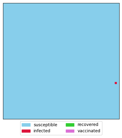
For our first scenario, we create a model with only one infected person and observe how the disease spreads. First, we create a model with the default parameters modifying only the number of infected people at the start and look at the initial state.

sim = EpisimCA(start_num_infected=1)
print(f"Population: {sim.num_people} (infected: {sim.num_infected}, vaccinated: {sim.num_vaccinated})")
sim.plot_grid()

Population: 2500 (infected: 1, vaccinated: 0)

Now we update the state of the grid with the update rule described above. We do this 75 times and create an animation of the evolution of our grid.

def animate(it, simulation, neighbourhood="Neumann"):
    """
    runs one simulation update step and adds a plot to the animation.
    To be used within FuncAnimation
    :param it: iteration count (currently unused)
    :param simulation: simulation object
    :param neighbourhood: neigbourhood type as supported by the simulation
    """
    simulation.update(neighbourhood=neighbourhood)
    simulation.plot_state(animate=True)
plt.figure(figsize=(10, 5))
anim = animation.FuncAnimation(plt.gcf(), animate, frames = 150, interval = 100, 
                               fargs=(sim, "Neumann"))
video = HTML(anim.to_jshtml())
plt.close()
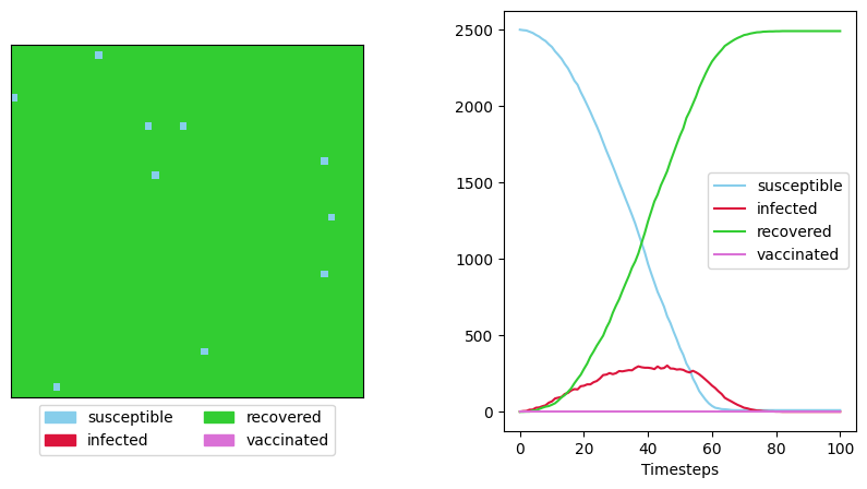
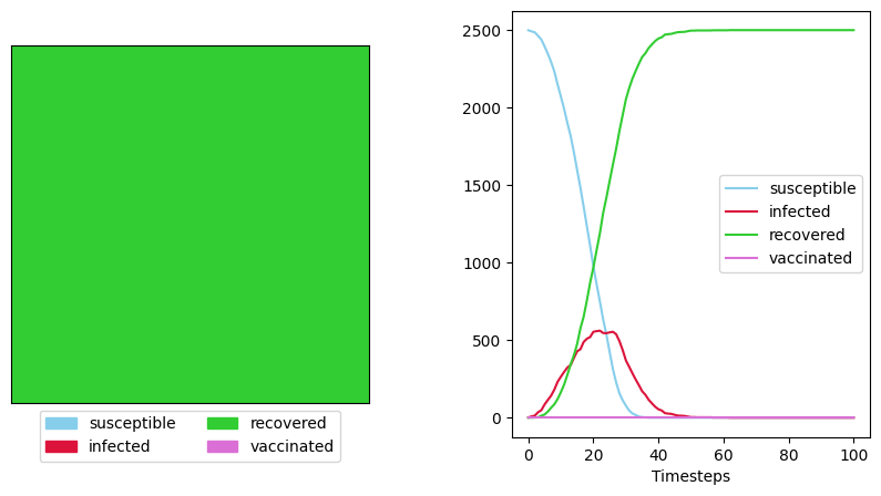
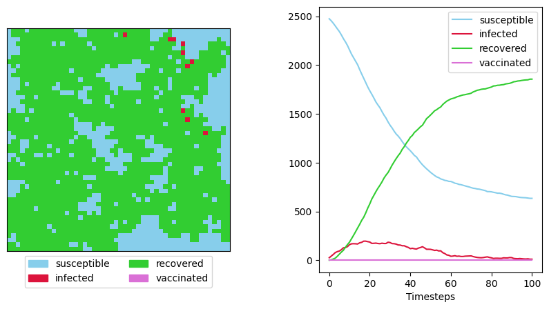
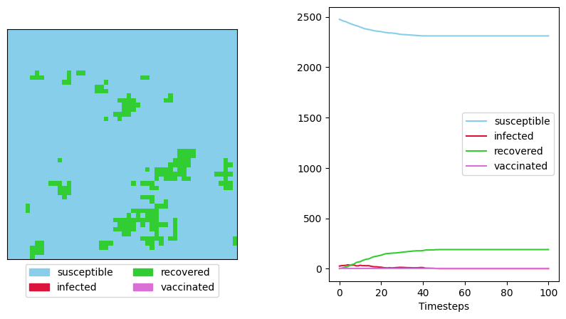
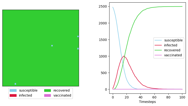
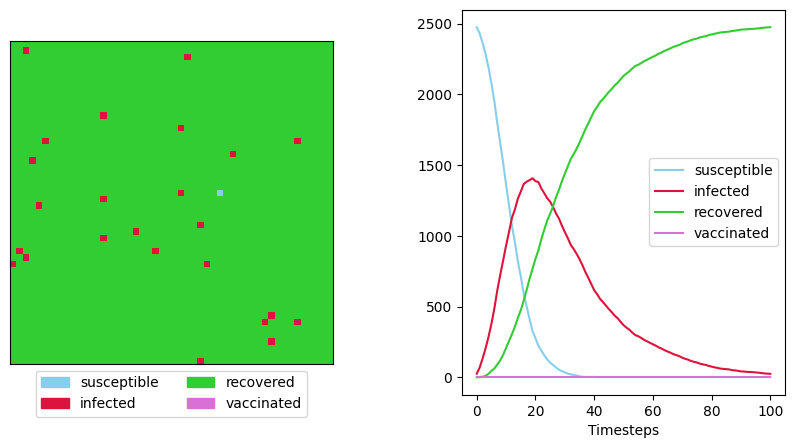
video # display the video object

Scenario 2: Different Neighbourhoods¶

When looking at Figure 1 it is immediately obvious how the different neighbourhoods can be interpreted. The more neighbours we take into account for our update rule, the faster the infections spreads. Also, the chance that a susceptible cell never gets infected shrinks significantly with larger neighbourhoods.

sim_neumann = EpisimCA(start_num_infected=1)
sim_moore = copy.deepcopy(sim_neumann)
sim_dist = copy.deepcopy(sim_neumann)

for _ in range(100):
    sim_neumann.update(neighbourhood="Neumann")
    sim_moore.update(neighbourhood="Moore")
    sim_dist.update(neighbourhood="distance")

sim_neumann.plot_state()
sim_moore.plot_state()
sim_dist.plot_state()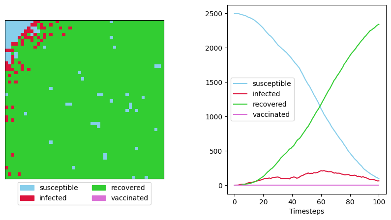

Scenario 3: Large Population¶

A big advantage of cellular automatas is that they are easy to compute if efficiently implemented. For example, for our next scenario, we create a model with a population of 250000 and 500 infected people at the start. Even though this is a very large population, simulating 50 timesteps takes only a few miliseconds.

sim_large = EpisimCA(grid_dimensions=(500, 500), start_num_infected=500)
for _ in range(75):
    sim_large.update()
sim_large.plot_stats(figsize=(8, 5));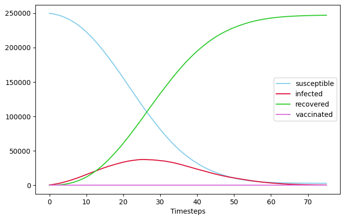

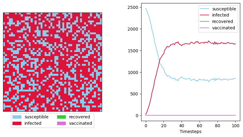
Scenario 4: Varying Parameters¶

Now lets have a look at how changing the model parameter influences the outcomes.

First, we vary the infection probability. Up until now, we used the default value of 0.4. In the next cell, we create three models with different infection probabilities that are otherwise identical in their parameters. And observer their state after 100 timespteps.

sim_1 = EpisimCA(infection_probability=0.6)
sim_2 = EpisimCA(infection_probability=0.2)
sim_3 = EpisimCA(infection_probability=0.1)

for _ in range(100):
    sim_1.update()
    sim_2.update()
    sim_3.update()

sim_1.plot_state()
sim_2.plot_state()
sim_3.plot_state()

We observe that the with lower infection probability, the simulation takes longer to reach an equilibrium. Additionally, we observe that lower infection probabilities lead to more people never getting infected. This makes sense, as infected people are less likely to infect others before the recover.

Now consider how the recovery probability affects our results. In the next cell, we create models with different recovery probabilities from our default of $p_r=0.2$ and observe the state of the model after 100 timesteps.

sim_1 = EpisimCA(recovery_probability=0.4)
sim_2 = EpisimCA(recovery_probability=0.1)
sim_3 = EpisimCA(recovery_probability=0.05)

for _ in range(100):
    sim_1.update()
    sim_2.update()
    sim_3.update()

sim_1.plot_state()
sim_2.plot_state()
sim_3.plot_state()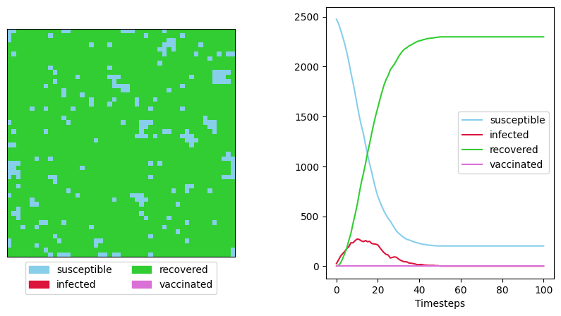

We see a kind of similar pattern as before. Again, lower recovery probabilities lead to a longer time to reach an equilibrium. Also, we can see the peak of infected people is rising with lower recovery probabilities because it takes longer for people to recover once they are infected.

Scenario 5: SIS Model¶

For this scenario we have a look at the SIS model type. With this model type we omit the recovered state of the cell. Instead, an infected cell will go back to being susceptible after being infected and can become infected again.

sim = EpisimCA(model_type="SIS")
plt.figure(figsize=(10, 5))
anim = animation.FuncAnimation(plt.gcf(), animate, frames = 50, interval = 333, 
                               fargs=(sim, "Neumann"))
video = HTML(anim.to_jshtml())
plt.close()
video

We will reach an equilibrium of infected and susceptible cells. The ration of infected to susceptible cells at the equilibrium can be adjusted by changing the ratio of infection probability to recovery probability.

sim_1 = EpisimCA(model_type="SIS", infection_probability=0.4, recovery_probability=0.4)  # ratio 1 : 1
sim_2 = EpisimCA(model_type="SIS", infection_probability=0.4, recovery_probability=0.2)  # ratio 2 : 1
sim_3 = EpisimCA(model_type="SIS", infection_probability=0.2, recovery_probability=0.4)  # ratio 1 : 2

for _ in range(100):
    sim_1.update()
    sim_2.update()
    sim_3.update()

sim_1.plot_state()
sim_2.plot_state()
sim_3.plot_state()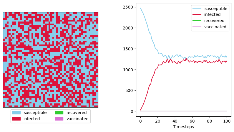

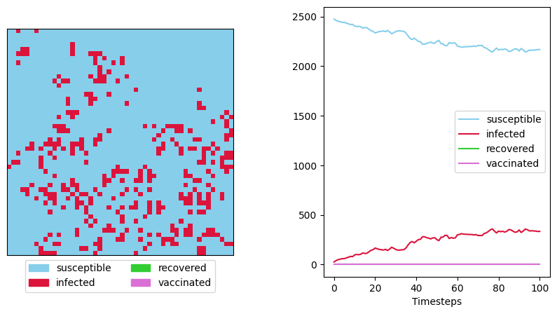
Scenario 6: Introducing Vaccinations¶

For the last scenario we introduce vaccinations into our model by setting $p_v>0$ .

sim = EpisimCA(vaccination_probability=0.1)
plt.figure(figsize=(10, 5))
anim = animation.FuncAnimation(plt.gcf(), animate, frames = 50, interval = 500, 
                               fargs=(sim, "Moore"))
video = HTML(anim.to_jshtml())
plt.close()
video

As expected, vaccination lead to less cells getting infected. Perhaps more interestingly, we can see pattern emerge. Regions in proximity to the initial infections will still mostly get infected but if the vaccination probability is high enough the infections can get isolated, protecting whole clusters of cells from getting infected.

References¶

Bicher, M., & Popper, N. (2013). Agent-Based Derivation of the SIR-Differential Equations. 2013 8th EUROSIM Congress on Modelling and Simulation. 10.1109/eurosim.2013.62